Wannier90 Silicon example

from pythtb import W90
import matplotlib.pyplot as plt
import numpy as np

silicon = W90("silicon_w90", "si")

# hard coded fermi level in eV
fermi_ev = 6.2285135

# all pair distances between the orbitals
print("Shells:\n", silicon.shells())

Shells:
 [ 0.    1.3   1.96  2.35  2.51  2.97  3.18  3.36  3.66  3.82  3.93  4.03
  4.29  4.48  4.57  4.61  4.83  4.97  5.12  5.29  5.32  5.4   5.42  5.48
  5.52  5.55  5.74  5.89  5.95  6.13  6.16  6.27  6.33  6.36  6.39  6.52
  6.55  6.61  6.63  6.74  6.89  7.07  7.1   7.22  7.25  7.39  7.44  7.56
  7.58  7.63  7.69  7.72  7.74  7.77  7.88  7.9   7.99  8.04  8.17  8.19
  8.27  8.31  8.32  8.34  8.36  8.47  8.49  8.53  8.55  8.59  8.74  8.78
  8.81  8.85  8.92  8.94  9.02  9.11  9.15  9.19  9.31  9.35  9.36  9.44
  9.46  9.53  9.55  9.57  9.64  9.72  9.79  9.81  9.88  9.92 10.04 10.29
 10.3  10.4  10.44 10.52 10.54 10.62 10.76 10.8  10.84 10.87 10.99 11.08
 11.18 11.21 11.26 11.29 11.38 11.46 11.72 11.75 12.23 12.24 12.43 13.08
 13.2  13.28 13.45]

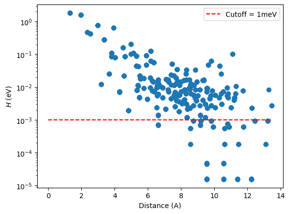
We can look at how the Hamiltonian matrix elements generated by Wannier90 decay with distance. This will help us determine the cutoff radius to use in a tight-binding model constructed with pythtb. Most hoppings are above \(1\) meV, so we will use this as our curtoff energy in this example.

# plot hopping terms as a function of distance on a log scale
(dist, ham) = silicon.dist_hop()
fig, ax = plt.subplots()
ax.scatter(dist, np.abs(ham))
ax.hlines(
    1e-3, xmin=0, xmax=max(dist), colors="r", linestyles="dashed", label="Cutoff = 1meV"
)
ax.legend()
ax.set_xlabel("Distance (A)")
ax.set_ylabel(r"$H$ (eV)")
ax.set_yscale("log")

Now, we will generate the tight-binding model for silicon using the Wannier90 output files. This will use the Hamiltonian matrix elements generated by Wannier90 to create a TBModel object in pythtb.

Tip

It is advised to save the tight-binding model to disk with the cPickle module:

import cPickle
cPickle.dump(my_model, open("store.pkl", "wb"))

Later one can load in the model from disk in a separate script with

my_model = cPickle.load(open("store.pkl", "rb"))

# get tb model in which some small terms are ignored
my_model = silicon.model(
    zero_energy=fermi_ev,
    min_hopping_norm=1e-3,
)

Band comparison

First, we will obtain the band structure from the Wannier90 calculation. To do this, we call the W90.w90_bands function, which reads the si_band.dat, si_band.kpt and si.win files to extract the band energies and k-point path used in the Wannier90 calculation. Setting return_k_dist = True returns the cumulative distance along the k-point path, which we will use for plotting. Setting return_k_nodes = True returns the fractional coordinates of the high-symmetry k-points along the path, as well as their labels.

Hint

Small discrepancies in the plot may arise due to the terms that were ignored in the silicon.model function call above.

(w90_kpt, w90_evals, w90_k_dist, w90_k_nodes, w90_k_labels) = silicon.bands_w90(
    return_k_dist=True, return_k_nodes=True
)

print("k-point labels:", w90_k_labels)
print("k-point nodes (fractional):\n", w90_k_nodes)

k-point labels: ['$L$', '$\\Gamma$', '$X$', '$X$', '$K$', '$\\Gamma$']
k-point nodes (fractional):
 [[ 0.5    0.5    0.5  ]
 [ 0.     0.     0.   ]
 [ 0.5    0.     0.5  ]
 [ 0.5   -0.5    0.   ]
 [ 0.375 -0.375  0.   ]
 [ 0.     0.     0.   ]]

For plotting purposes, we also need to know the cumulative distance along the k-point path at each high-symmetry k-point node, which we compute below.

k_vec, k_dist, k_node_dist = my_model.k_path(w90_k_nodes, nk=500, report=False)

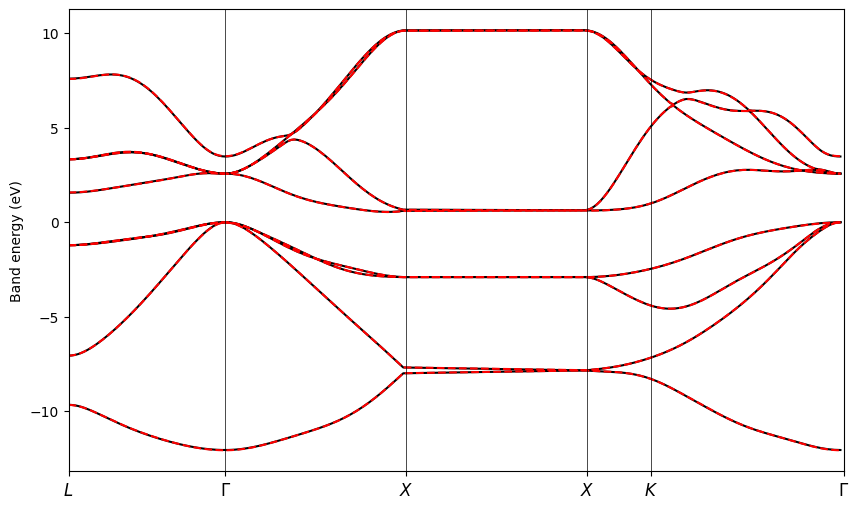
Next, we will solve and plot the TBModel on the same path as used in Wannier90. This allows us to directly compare the two band structures.

int_evals = my_model.solve_ham(w90_kpt)

fig, ax = plt.subplots(figsize=(10, 6))

ax.plot(w90_k_dist, w90_evals[:, 0] - fermi_ev, "k-", zorder=0, label="Wannier90")
ax.plot(w90_k_dist, w90_evals[:, 1:] - fermi_ev, "k-", zorder=0)
ax.plot(w90_k_dist, int_evals[:, 0], "r--", zorder=1, label="TBModel")
ax.plot(w90_k_dist, int_evals[:, 1:], "r--", zorder=1)

# set x-ticks at k-point nodes
ax.set_xticks(k_node_dist)
for n in range(len(w90_k_nodes)):
    ax.axvline(x=k_node_dist[n], linewidth=0.5, color="k", zorder=1)
ax.set_xticklabels(w90_k_labels, size=12)
ax.set_xlim(k_node_dist[0], k_node_dist[-1])
ax.set_ylabel("Band energy (eV)")
plt.show()