tb_model to TBModel in v2.0#
This notebook will walk you through some of the important changes to the tb_model class in v2.0. For a more comprehensive overview of all changes, please refer to the release notes.
The first thing to be aware of is that the module names have changed
< v1.8:
tb_model,wf_array,w902.0:
TBModel,WFArray,W90
This needs to be changed at the import line
from pythtb import TBModel, Lattice
import numpy as np
Constructing a TBModel#
The construction of the model has changed in v2.0. Instead of passing the lattice vectors and orbital positions as separate arguments, we now pass a Lattice object that contains this information.
We will build use a honeycomb lattice as an example. In v1.8, we would do this as follows:
# v1.8 code
from pythtb import tb_model

lat_vecs = [[1, 0], [1/2, np.sqrt(3) / 2]]
orb_vecs = [[1/3, 1/3], [2/3, 2/3]]
model = tb_model(dim_r = 2, dim_k = 2, lat=lat_vecs, orb=orb_vecs, per=[0,1], nspin=1)
In v2.0, we first create a Lattice object and then pass it to the TBModel constructor.
A few behavioral changes to note:
peris now namedperiodic_dirsfor clarity. If not specified, default behavior in v1.8 was to assume all directions were periodic; in v2.0, the default is no periodic directions.The
nspininteger argument has been replaced withspinful, a boolean that indicates whether the model is spinful or spinless.dim_randdim_kare no longer required arguments, as they can be inferred from thelat_vecsandperiodic_dirs.
Everything else remains mostly the same, just wrapped in a Lattice object.
Tip
A convenient way to specify all lattice directions as periodic is to use ... for the periodic_dirs argument, e.g. periodic_dirs=....
Alternatively, you can also pass periodic_dirs="all" to achieve the same effect.
Here is the equivalent code in v2.0:
lat_vecs = [[1, 0], [1 / 2, np.sqrt(3) / 2]]
orb_vecs = [[1 / 3, 1 / 3], [2 / 3, 2 / 3]]
lat = Lattice(lat_vecs=lat_vecs, orb_vecs=orb_vecs, periodic_dirs=[0, 1])
model = TBModel(lattice=lat, spinful=False)
delta = 0
t1 = -1
t2 = 0.15
phi = np.pi / 2

model.set_onsite([-delta, delta], mode="set")

for lvec in ([0, 0], [-1, 0], [0, -1]):
    model.set_hop(t1, 0, 1, lvec, mode="set")

for lvec in ([1, 0], [-1, 1], [0, -1]):
    model.set_hop(t2 * np.exp(1j * phi), 0, 0, lvec, mode="set")
for lvec in ([-1, 0], [1, -1], [0, 1]):
    model.set_hop(t2 * np.exp(1j * phi), 1, 1, lvec, mode="set")
models library#
A collection of TBModel generators for prototypical tight-binding models has been included in pythtb.models. The models are
checkerboard
haldane
kane-mele
graphene
As an example, we can import the same Haldane tight-binding model as used above from the models library:
from pythtb.models import haldane

my_model = haldane(delta=0.1, t1=1.0, t2=0.1)
Reporting the model information#
To see the model information, previously one would call
# v1.8
my_model.display()
In v2.0, display is now called info. An alternative way of seeing the same information is to simply print the model
# v2.0
print(my_model)
# or
my_model.info()
print(my_model)
----------------------------------------
       Tight-binding model report
----------------------------------------
r-space dimension           = 2
k-space dimension           = 2
periodic directions         = [0, 1]
spinful                     = False
number of spin components   = 1
number of electronic states = 2
number of orbitals          = 2

Lattice vectors (Cartesian):
  # 0 ===> [ 1.000,  0.000]
  # 1 ===> [ 0.500,  0.866]
Volume of unit cell (Cartesian) = 0.866 [A^d]

Reciprocal lattice vectors (Cartesian):
  # 0 ===> [ 6.283, -3.628]
  # 1 ===> [ 0.000,  7.255]
Volume of reciprocal unit cell = 45.586 [A^-d]

Orbital vectors (Cartesian):
  # 0 ===> [ 0.500,  0.289]
  # 1 ===> [ 1.000,  0.577]

Orbital vectors (fractional):
  # 0 ===> [ 0.333,  0.333]
  # 1 ===> [ 0.667,  0.667]
----------------------------------------
Site energies:
  < 0 | H | 0 > = -0.100
  < 1 | H | 1 > =  0.100
Hoppings:
  < 0 | H | 1  + [ 0.0 ,  0.0 ] > = 1.0000+0.0000j
  < 0 | H | 1  + [-1.0 ,  0.0 ] > = 1.0000+0.0000j
  < 0 | H | 1  + [ 0.0 , -1.0 ] > = 1.0000+0.0000j
  < 0 | H | 0  + [ 1.0 ,  0.0 ] > = 0.0000+0.1000j
  < 0 | H | 0  + [-1.0 ,  1.0 ] > = 0.0000+0.1000j
  < 0 | H | 0  + [ 0.0 , -1.0 ] > = 0.0000+0.1000j
  < 1 | H | 1  + [-1.0 ,  0.0 ] > = 0.0000+0.1000j
  < 1 | H | 1  + [ 1.0 , -1.0 ] > = 0.0000+0.1000j
  < 1 | H | 1  + [ 0.0 ,  1.0 ] > = 0.0000+0.1000j
Hopping distances:
  | pos( 0 ) - pos( 1 ) + [ 0.0 ,  0.0 ] | =   0.577
  | pos( 0 ) - pos( 1 ) + [-1.0 ,  0.0 ] | =   0.577
  | pos( 0 ) - pos( 1 ) + [ 0.0 , -1.0 ] | =   0.577
  | pos( 0 ) - pos( 0 ) + [ 1.0 ,  0.0 ] | =   1.000
  | pos( 0 ) - pos( 0 ) + [-1.0 ,  1.0 ] | =   1.000
  | pos( 0 ) - pos( 0 ) + [ 0.0 , -1.0 ] | =   1.000
  | pos( 1 ) - pos( 1 ) + [-1.0 ,  0.0 ] | =   1.000
  | pos( 1 ) - pos( 1 ) + [ 1.0 , -1.0 ] | =   1.000
  | pos( 1 ) - pos( 1 ) + [ 0.0 ,  1.0 ] | =   1.000
Visualizing the tight-binding model#
The visualization of the tight-binding model orbital positions and hopping bonds has been updated. As before we call my_model.visualize in order see the tight-binding lattice.
In v1.8, one would use:
# v1.8
my_model.visualize(0, 1)
The resulting plot would look like this:
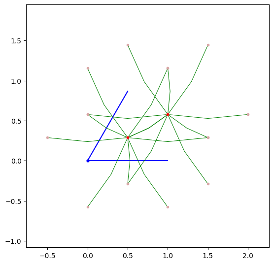
The difference here is that we no longer have to specify the lattice directions to plot in 2D. In 3D, we still can specify the proj_plane argument with two integers corresponding to \(a_i\) and \(a_j\) lattice vectors, onto which to project the 3D structure. The default behavior is to plot in 2D for 2D models, and to project onto the \(a_1\)-\(a_2\) plane for 3D models.
..note::
For 3D models, we can now plot the three-dimensional structure using visualize3d() if plotly is installed.
In v2.0, the output looks like this:
my_model.visualize()
(<Figure size 800x800 with 1 Axes>, <Axes: xlabel='x', ylabel='y'>)
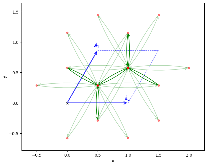
Notice that the hoppings are not all the same boldness. The alpha values of the bonds are scaled according to the hopping strength. Additionally, we can now annotate the onsite energies by setting the annotate_onsite_en argument to True.
Accessing the Hamiltonian matrix#
In previous versions of pythtb, one could not directly access the Hamiltonian matrix. Instead, one would call my_model.solve_all(kpts) or my_model.solve_one(kpt) to get the eigenvalues and eigenvectors at a given k-point. In v2.0, we can now directly access the Hamiltonian matrix at a list of k-points using my_model.hamiltonian(kpts), which returns a NumPy array.
# Generate k-points
nkx, nky = 20, 20
k_pts = my_model.k_uniform_mesh([nkx, nky])
H_k = my_model.hamiltonian(k_pts)

print("Hamiltonian shape:", H_k.shape)
print("Hamiltonian at first k-point:\n", H_k[0])
print("Hamiltonian at second k-point:\n", H_k[1])
Hamiltonian shape: (400, 2, 2)
Hamiltonian at first k-point:
 [[-0.1+0.j  3. +0.j]
 [ 3. +0.j  0.1+0.j]]
Hamiltonian at second k-point:
 [[-0.1       -5.00594829e-34j  2.96365774+1.33535078e-03j]
 [ 2.96365774-1.33535078e-03j  0.1       +6.90854711e-35j]]
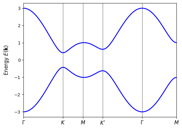
Band plotting#
A new feature to TBModel’s is a convience function for quickly plotting band structures. Instead of explictly creating the k-path and making the matplotlib figure, we can just call plot_bands and pass the high-symmetry points in reduced units. This will return the matplotlib figure and axis objects for further customization.
Note
We may also pass the k_node_labels argument to specify the labels for the high-symmetry points.
Compare this with v1.8:
# v1.8 code
path=[[0.,0.],[2./3.,1./3.],[.5,.5],[1./3.,2./3.], [0.,0.]]
label=(r'$\Gamma $',r'$K$', r'$M$', r'$K^\prime$', r'$\Gamma $')

(k_vec,k_dist,k_node) = my_model.k_path(path,101)
evals = my_model.solve_all(k_vec)

fig, ax = plt.subplots()
ax.set_xlim(k_node[0],k_node[-1])
ax.set_xticks(k_node)
ax.set_xticklabels(label)
for n in range(len(k_node)):
  ax.axvline(x=k_node[n],linewidth=0.5, color='k')
ax.set_ylabel("Band energy")

ax.plot(k_dist,evals[0])
ax.plot(k_dist,evals[1])
k_nodes = [[0, 0], [2 / 3, 1 / 3], [0.5, 0.5], [1 / 3, 2 / 3], [0, 0], [0.5, 0.5]]
k_label = (r"$\Gamma $", r"$K$", r"$M$", r"$K^\prime$", r"$\Gamma $", r"$M$")

fig, ax = my_model.plot_bands(k_nodes=k_nodes, k_node_labels=k_label)
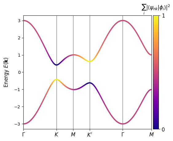
An optional flag allows one to visualize the orbital character of the bands. To do so, we provide a list to proj_orb_idx. The list defines the indices of the orbitals to project the eigenstates onto. This will show a colorbar displaying the weight of the eigenstates onto that set of orbitals.
In this example, the Haldane model demonstrates a band inversion at the \(K\) and \(K'\) points, a hallmark of the topological phase transition.
fig, ax = my_model.plot_bands(
    nk=500, k_nodes=k_nodes, k_node_labels=k_label, proj_orb_idx=[1]
)
Backwards Compatibility#
To maintain backwards compatibility with scripts written for PythTB v1.8 and earlier, the old tb_model is still available as an alias to TBModel. The functions and methods will be from v2.0, but the old way of initializing the tb_model class will still work.
from pythtb import tb_model
import numpy as np
From v1.8.0 Haldane model initialization:
# define lattice vectors
lat = [[1.0, 0.0], [0.5, np.sqrt(3.0) / 2.0]]
# define coordinates of orbitals
orb = [[1.0 / 3.0, 1.0 / 3.0], [2.0 / 3.0, 2.0 / 3.0]]

# make two dimensional tight-binding Haldane model
my_model = tb_model(2, 2, lat, orb)

# set model parameters
delta = 0.2
t = -1.0
t2 = 0.15 * np.exp((1.0j) * np.pi / 2.0)
t2c = t2.conjugate()

# set on-site energies
my_model.set_onsite([-delta, delta])
# set hoppings (one for each connected pair of orbitals)
# (amplitude, i, j, [lattice vector to cell containing j])
my_model.set_hop(t, 0, 1, [0, 0])
my_model.set_hop(t, 1, 0, [1, 0])
my_model.set_hop(t, 1, 0, [0, 1])
# add second neighbour complex hoppings
my_model.set_hop(t2, 0, 0, [1, 0])
my_model.set_hop(t2, 1, 1, [1, -1])
my_model.set_hop(t2, 1, 1, [0, 1])
my_model.set_hop(t2c, 1, 1, [1, 0])
my_model.set_hop(t2c, 0, 0, [1, -1])
my_model.set_hop(t2c, 0, 0, [0, 1])

# print tight-binding model
my_model.display()
----------------------------------------
       Tight-binding model report
----------------------------------------
r-space dimension           = 2
k-space dimension           = 2
periodic directions         = [0, 1]
spinful                     = False
number of spin components   = 1
number of electronic states = 2
number of orbitals          = 2

Lattice vectors (Cartesian):
  # 0 ===> [ 1.000,  0.000]
  # 1 ===> [ 0.500,  0.866]
Volume of unit cell (Cartesian) = 0.866 [A^d]

Reciprocal lattice vectors (Cartesian):
  # 0 ===> [ 6.283, -3.628]
  # 1 ===> [ 0.000,  7.255]
Volume of reciprocal unit cell = 45.586 [A^-d]

Orbital vectors (Cartesian):
  # 0 ===> [ 0.500,  0.289]
  # 1 ===> [ 1.000,  0.577]

Orbital vectors (fractional):
  # 0 ===> [ 0.333,  0.333]
  # 1 ===> [ 0.667,  0.667]
----------------------------------------
Site energies:
  < 0 | H | 0 > = -0.200
  < 1 | H | 1 > =  0.200
Hoppings:
  < 0 | H | 1  + [ 0.0 ,  0.0 ] > = -1.0000+0.0000j
  < 1 | H | 0  + [ 1.0 ,  0.0 ] > = -1.0000+0.0000j
  < 1 | H | 0  + [ 0.0 ,  1.0 ] > = -1.0000+0.0000j
  < 0 | H | 0  + [ 1.0 ,  0.0 ] > = 0.0000+0.1500j
  < 1 | H | 1  + [ 1.0 , -1.0 ] > = 0.0000+0.1500j
  < 1 | H | 1  + [ 0.0 ,  1.0 ] > = 0.0000+0.1500j
  < 1 | H | 1  + [ 1.0 ,  0.0 ] > = 0.0000-0.1500j
  < 0 | H | 0  + [ 1.0 , -1.0 ] > = 0.0000-0.1500j
  < 0 | H | 0  + [ 0.0 ,  1.0 ] > = 0.0000-0.1500j
Hopping distances:
  | pos( 0 ) - pos( 1 ) + [ 0.0 ,  0.0 ] | =   0.577
  | pos( 1 ) - pos( 0 ) + [ 1.0 ,  0.0 ] | =   0.577
  | pos( 1 ) - pos( 0 ) + [ 0.0 ,  1.0 ] | =   0.577
  | pos( 0 ) - pos( 0 ) + [ 1.0 ,  0.0 ] | =   1.000
  | pos( 1 ) - pos( 1 ) + [ 1.0 , -1.0 ] | =   1.000
  | pos( 1 ) - pos( 1 ) + [ 0.0 ,  1.0 ] | =   1.000
  | pos( 1 ) - pos( 1 ) + [ 1.0 ,  0.0 ] | =   1.000
  | pos( 0 ) - pos( 0 ) + [ 1.0 , -1.0 ] | =   1.000
  | pos( 0 ) - pos( 0 ) + [ 0.0 ,  1.0 ] | =   1.000
/tmp/ipykernel_1294/2945160337.py:7: DeprecationWarning: pythtb.tb_model is deprecated and will be removed in a future release. Use TBModel instead.
  my_model = tb_model(2, 2, lat, orb)
/tmp/ipykernel_1294/2945160337.py:31: FutureWarning: TBModel.display is deprecated and will be removed in a future release: The 'display()' method is deprecated and will be removed in a future release. Use 'print(model)' or 'model.info(show=True)' instead.
  my_model.display()
Other new features#
Explore the variety of new methods available in the TBModel class in v2.0 by checking out the API documentation and the following tutorials: