Axion angle of the Fu-Kane-Mele pump#
The axion angle \(\theta\) characterizes the isotropic magnetoelectric response of a three-dimensional insulator. When \(\theta\) evolves adiabatically along a closed cycle of a control parameter \(\lambda\), its change is quantized and proportional to the second Chern number of the occupied bands. This is the 4D analogue of Thouless charge pumping: just as a 1D insulator pumps an integer charge over a cycle (first Chern number), a 3D insulator can pump a quantized axion angle governed by a second-Chern invariant.
In this notebook, we show how pythtb can be used to compute \(\theta(\lambda)\). TBModel.axion_angle evaluates \(\theta(\lambda)\) using the four-curvature formulation
Here, \(\Omega_{\mu\nu}\) is the non-Abelian Berry curvature defined in 4D space \((k_x,k_y,k_z,\lambda)\). This integrand is gauge-invariant, and provided the gap remains open along the path, the total change in \(\theta\) over a closed cycle is quantized to \(2\pi C_2\), where \(C_2\) is the second Chern number.
Gauge-dependent formulation of \(\theta\)
Alternatively, the axion angle can be computed using the Chern-Simons 3-form,
where \(\mathcal{A}_i\) is the non-Abelian Berry connection. This expression is gauge-dependent and requires a constructing a smooth gauge over the entire Brillouin zone.
The method implemented here does not perform such gauge fixing and does not evaluate this Chern-Simons form directly. Instead, TBModel.axion_angle integrates a gauge-invariant four-curvature along an adiabatic path beginning from a reference configuration with a known \(\theta=0\), yielding the relative quantity \(\theta(\lambda) - \theta(0)\). This approach avoids gauge-fixing while still capturing the quantized \(2\pi\) winding over a closed cycle when the gap remains open.
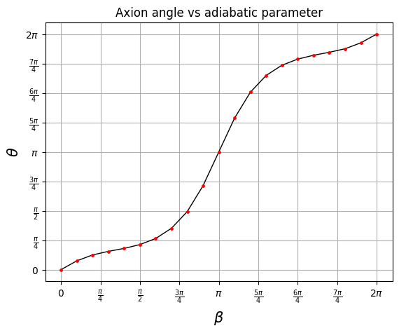
As an example, we study the Fu-Kane-Mele (FKM) model on a diamond lattice, a canonical three-dimensional topological insulator. In the presence of time-reversal and inversion symmetry, the axion angle is quantized to either 0 or \(\pi\) (mod \(2\pi\)), corresponding to trivial and non-trivial topological phases, respectively. Introducing an adiabatic parameter \(\beta\) breaks these symmetries for \(\beta \neq n \pi\), allowing \(\theta(\beta)\) to vary continuously between these quantized limits. We sweep \(\beta\) over a \(2\pi\) cycle, compute \(\theta(\beta)\) using TBModel.axion_angle, and verify the expected \(2\pi\) pump corresponding to a unit second Chern number.
What you will learn
Setting up a three-dimensional model with an adiabatic parameter.
How to compute the axion angle as a function of an adiabatic parameter using
TBModel.axion_angle.How to compute the second Chern number associated with the adiabatic cycle.
import numpy as np
from pythtb import TBModel, Lattice
import matplotlib.pyplot as plt
Fu-Kane-Mele model setup#
We use a lambda function to define the FKM model with an adiabatic parameter beta. The parameter beta enters as a staggered Zeeman field and first-neighbor hopping modulation along \((111)\) that gaps the Dirac nodes.
lat_vecs = [[0, 1, 1], [1, 0, 1], [1, 1, 0]]
orb_vecs = [[0, 0, 0], [0.25, 0.25, 0.25]]
lat = Lattice(lat_vecs, orb_vecs, periodic_dirs=...)

model = TBModel(lattice=lat, spinful=True)

# fixed parameters
t = 1.0
soc = 1 / 4
m = 1 / 2

# Staggered Zeeman term along (111)
# same magnitude for sigma_x,y,z on each site with opposite sign on the two sites
model.set_onsite(
    lambda beta: [0, m * np.sin(beta), m * np.sin(beta), m * np.sin(beta)],
    ind_i=0,
)  # site 0
model.set_onsite(
    lambda beta: [0, -m * np.sin(beta), -m * np.sin(beta), -m * np.sin(beta)],
    ind_i=1,
)  # site 1

# spin-independent first-neighbor hops
for lvec in ([-1, 0, 0], [0, -1, 0], [0, 0, -1]):
    model.set_hop(t, 0, 1, lvec)

# modulated first-neighbor hop along (111)
model.set_hop(lambda beta: 3 * t + m * np.cos(beta), 0, 1, [0, 0, 0], mode="set")

# spin-dependent second-neighbor hops
lvec_list = ([1, 0, 0], [0, 1, 0], [0, 0, 1], [-1, 1, 0], [0, -1, 1], [1, 0, -1])
dir_list = ([0, 1, -1], [-1, 0, 1], [1, -1, 0], [1, 1, 0], [0, 1, 1], [1, 0, 1])
for j in range(6):
    spin = np.array([0.0] + dir_list[j])
    model.set_hop(1j * soc * spin, 0, 0, lvec_list[j])
    model.set_hop(-1j * soc * spin, 1, 1, lvec_list[j])

print(model)
Computing the axion angle#
We first define our set of sampling points in \(\beta\) and k-space. The k-space grid is computed automatically from the specified nks in the TBModel.axion_angle as a uniform reduced grid with endpoints excluded. The \(\beta\) points are defined manually here.
For the adiabatic direction we supply an array of beta values covering a full \(2\pi\) cycle.
Including endpoints in a cyclic adiabatic parameter sweep
When defining a cyclic adiabatic parameter sweep, it is often convenient to include both endpoints of the cycle in the betas array to ensure that the returned \(\theta(\beta)\) also includes the endpoint value.
The choice to include or exclude the endpoints of the cycle in the betas array will not change the second Chern number returned by TBModel.axion_angle as long as we specify the periodicity of the cycle using param_periods. Internally, the code will trim these endpoints when integrating the second Chern number, and re-append them to the returned \(\theta(\beta)\). Specifying the periodicity is also necessary to ensure that the finite-difference stencil used to compute derivatives along the adiabatic direction respects the periodicity of the parameter. If left unspecified, the code will assume the parameter is non-periodic and use one-sided finite-difference stencils at the endpoints. The second Chern number in this case may generally be skewed by the inclusion of the additional endpoint if param_periods is left unspecified.
To make sure the finite-difference stencil respects the periodicity of \(\beta\), pass
param_periods = {"beta": 2*np.pi}
to TBModel.axion_angle (or whatever period applies).
nks = 40, 40, 40
n_beta = 21
betas = np.linspace(0, 2 * np.pi, n_beta, endpoint=True)
param_periods = {"beta": 2 * np.pi}

print(f"Total number of points: {nks[0] * nks[1] * nks[2] * n_beta}")
Total number of points: 1344000
Next, we call TBModel.axion_angle to compute the axion angle as a function of \(\beta\). The routine returns both the cumulative axion angle and, if requested, the second Chern number accumulated over a full period.
Note
TBModel.axion_angleutilizes the non-Abelian Berry curvature on the four-dimensional mesh \((k_x,k_y,k_z,\beta)\) as shown in the equation above. The Berry curvature is computed using the Kubo formula in terms of the velocity operators (seeTBModel.velocity) and the eigenvalues and eigenvectors of the Hamiltonian. This requires a global gap throughout the adiabatic cycle.The curvature components with respect to crystal momentum are obtained analytically from the tight-binding model, while derivatives along the swept parameter rely on the requested finite-difference stencil. We specify the derivative scheme and order using the
diff_schemeanddiff_orderarguments.
Speedup calculation
The computation of the 4-curvature can be computationally intensive, especially for large k-point grids and many \(\beta\) points. We set use_tensorflow = True to leverage TensorFlow for efficient computation. This can significantly speed up the calculation, especially when using a GPU.
betas, axion, c2 = model.axion_angle(
    nks=nks,
    param_periods=param_periods,
    return_second_chern=True,
    use_tensorflow=True,
    diff_scheme="central",
    diff_order=8,
    beta=betas,
)
WARNING: All log messages before absl::InitializeLog() is called are written to STDERR
I0000 00:00:1779816401.565091     778 cudart_stub.cc:31] Could not find cuda drivers on your machine, GPU will not be used.
I0000 00:00:1779816402.444756     778 cpu_feature_guard.cc:227] This TensorFlow binary is optimized to use available CPU instructions in performance-critical operations.
To enable the following instructions: AVX2 FMA, in other operations, rebuild TensorFlow with the appropriate compiler flags.
WARNING: All log messages before absl::InitializeLog() is called are written to STDERR
I0000 00:00:1779816404.654861     778 cudart_stub.cc:31] Could not find cuda drivers on your machine, GPU will not be used.
E0000 00:00:1779816405.309857     778 cuda_platform.cc:52] failed call to cuInit: INTERNAL: CUDA error: Failed call to cuInit: UNKNOWN ERROR (303)
W0000 00:00:1779816405.312996     778 cpu_allocator_impl.cc:82] Allocation of 327680000 exceeds 10% of free system memory.
W0000 00:00:1779816405.634851     778 cpu_allocator_impl.cc:82] Allocation of 327680000 exceeds 10% of free system memory.
W0000 00:00:1779816408.208567     778 cpu_allocator_impl.cc:82] Allocation of 655360000 exceeds 10% of free system memory.
W0000 00:00:1779816409.047802     778 cpu_allocator_impl.cc:82] Allocation of 163840000 exceeds 10% of free system memory.
W0000 00:00:1779816409.265397 778 cpu_allocator_impl.cc:82] Allocation of 163840000 exceeds 10% of free system memory.
The second Chern number is also computed using the four-curvature field. The form is
Since \(\beta\) is periodic with period \(2\pi\), the second Chern number is expected to be an integer (up to numerical tolerance).
print(f"Second Chern number C2 = {c2}")
Second Chern number C2 = 1.00011146068573
At \(\beta =0, \pi, 2\pi\) the system is time-reversal symmetric, and the axion angle is quantized to 0 or \(\pi\) (mod \(2\pi\)). Away from these points the axion angle evolves smoothly. At \(\beta = \pi\), the system is in a topological insulator phase with axion angle \(\pi\). The cumulative result over a full \(2\pi\) cycle shows that the axion angle is pumped by \(2\pi\), consistent with the non-trivial topology of the adiabatic cycle. This corresponds to a second Chern number of 1 over the \((\mathbf{k}, \beta)\) space.
See also
For more details on this calculation, see Essin, Moore, Vanderbilt, PRL 102, 146805 (2009). Compare the figure above to Fig. 1 of the paper.
Next steps
Try excluding the endpoints in the
betasarray and see how things change.Experiment with different finite-difference schemes and orders to see how they affect the accuracy of the axion angle and second Chern number.