Haldane Chern-insulator model#
The Haldane model is a two-dimensional tight-binding model that exhibits topological properties. It is defined on a honeycomb lattice and includes complex next-nearest neighbor hopping terms. The model is characterized by a non-zero Chern number, which gives rise to the quantum anomalous Hall effect.
Here we will visualize the band structure and density of states of the Haldane model using the pythtb library.
from pythtb import TBModel, Lattice
import numpy as np
import matplotlib.pyplot as plt
The Lattice class#
We start by defining a Lattice object that contains information about
the lattice vectors and orbital positions. The Lattice class is defined in the pythtb.lattice module.
For the Haldane model, we have a two-dimensional lattice with two orbitals per unit cell. The lattice vectors are given by:
where \(a\) is the lattice constant, which for our model is set to 1.
The orbital positions are given in reduced coordinates. For example, the position of one of the orbitals in our case is specified by the reduced coordinates [1/3, 1/3]. The corresponding real-space position is obtained by multiplying the reduced coordinates by the lattice vectors:
where \(\mathbf{a}_{i}\) are the lattice vectors. Below we define the lattice vectors and orbital positions for the Haldane model.
# define lattice vectors
lat_vecs = [[1, 0], [1 / 2, np.sqrt(3) / 2]]
# define coordinates of orbitals
orb_vecs = [[1 / 3, 1 / 3], [2 / 3, 2 / 3]]
We then create a Lattice object using these definitions. The Lattice class takes as input the lattice vectors, orbital positions, and a list indicating which directions are periodic. In our case, both directions are periodic.
lat = Lattice(lat_vecs=lat_vecs, orb_vecs=orb_vecs, periodic_dirs=[0, 1])
print(lat)
----------------------------------------
       Lattice structure report
----------------------------------------
r-space dimension           = 2
k-space dimension           = 2
periodic directions         = [0, 1]
number of orbitals          = 2

Lattice vectors (Cartesian):
  # 0 ===> [ 1.000,  0.000]
  # 1 ===> [ 0.500,  0.866]
Volume of unit cell (Cartesian) = 0.866 [A^d]

Reciprocal lattice vectors (Cartesian):
  # 0 ===> [ 6.283, -3.628]
  # 1 ===> [ 0.000,  7.255]
Volume of reciprocal unit cell = 45.586 [A^-d]

Orbital vectors (Cartesian):
  # 0 ===> [ 0.500,  0.289]
  # 1 ===> [ 1.000,  0.577]

Orbital vectors (fractional):
  # 0 ===> [ 0.333,  0.333]
  # 1 ===> [ 0.667,  0.667]
----------------------------------------
The TBModel class#
Now we can pass this Lattice to the TBModel class to initialize our tight-binding model with the specified geometry. We also specify that we have a spinless model by setting nspin=1.
my_model = TBModel(lattice=lat, spinful=False)
Next, we need to specify the hopping parameters for the model. In the Haldane model, we have two types of hopping: intra-sublattice hopping (between orbitals on the same sublattice) and inter-sublattice hopping (between orbitals on different sublattices). We can define these hopping parameters as follows:
Warning
Once specifying the hopping from site \(i\) to site \(j + \mathbf{R}_{j}\) using the TBModel.set_hop method, it automatically specifies the hopping from site \(j\) to site \(i - \mathbf{R}\) as well.
delta = 0.2
t = -1.0
t2 = 0.15 * np.exp(1j * np.pi / 2)
t2c = t2.conjugate()

# set on-site energies
my_model.set_onsite([-delta, delta])
# set hoppings (one for each connected pair of orbitals)
# (amplitude, i, j, [lattice vector to cell containing j])
my_model.set_hop(t, 0, 1, [0, 0])
my_model.set_hop(t, 1, 0, [1, 0])
my_model.set_hop(t, 1, 0, [0, 1])
# add second neighbour complex hoppings
my_model.set_hop(t2, 0, 0, [1, 0])
my_model.set_hop(t2, 1, 1, [1, -1])
my_model.set_hop(t2, 1, 1, [0, 1])
my_model.set_hop(t2c, 1, 1, [1, 0])
my_model.set_hop(t2c, 0, 0, [1, -1])
my_model.set_hop(t2c, 0, 0, [0, 1])

print(my_model)
----------------------------------------
       Tight-binding model report
----------------------------------------
r-space dimension           = 2
k-space dimension           = 2
periodic directions         = [0, 1]
spinful                     = False
number of spin components   = 1
number of electronic states = 2
number of orbitals          = 2

Lattice vectors (Cartesian):
  # 0 ===> [ 1.000,  0.000]
  # 1 ===> [ 0.500,  0.866]
Volume of unit cell (Cartesian) = 0.866 [A^d]

Reciprocal lattice vectors (Cartesian):
  # 0 ===> [ 6.283, -3.628]
  # 1 ===> [ 0.000,  7.255]
Volume of reciprocal unit cell = 45.586 [A^-d]

Orbital vectors (Cartesian):
  # 0 ===> [ 0.500,  0.289]
  # 1 ===> [ 1.000,  0.577]

Orbital vectors (fractional):
  # 0 ===> [ 0.333,  0.333]
  # 1 ===> [ 0.667,  0.667]
----------------------------------------
Site energies:
  < 0 | H | 0 > = -0.200
  < 1 | H | 1 > =  0.200
Hoppings:
  < 0 | H | 1  + [ 0.0 ,  0.0 ] > = -1.0000+0.0000j
  < 1 | H | 0  + [ 1.0 ,  0.0 ] > = -1.0000+0.0000j
  < 1 | H | 0  + [ 0.0 ,  1.0 ] > = -1.0000+0.0000j
  < 0 | H | 0  + [ 1.0 ,  0.0 ] > = 0.0000+0.1500j
  < 1 | H | 1  + [ 1.0 , -1.0 ] > = 0.0000+0.1500j
  < 1 | H | 1  + [ 0.0 ,  1.0 ] > = 0.0000+0.1500j
  < 1 | H | 1  + [ 1.0 ,  0.0 ] > = 0.0000-0.1500j
  < 0 | H | 0  + [ 1.0 , -1.0 ] > = 0.0000-0.1500j
  < 0 | H | 0  + [ 0.0 ,  1.0 ] > = 0.0000-0.1500j
Hopping distances:
  | pos( 0 ) - pos( 1 ) + [ 0.0 ,  0.0 ] | =   0.577
  | pos( 1 ) - pos( 0 ) + [ 1.0 ,  0.0 ] | =   0.577
  | pos( 1 ) - pos( 0 ) + [ 0.0 ,  1.0 ] | =   0.577
  | pos( 0 ) - pos( 0 ) + [ 1.0 ,  0.0 ] | =   1.000
  | pos( 1 ) - pos( 1 ) + [ 1.0 , -1.0 ] | =   1.000
  | pos( 1 ) - pos( 1 ) + [ 0.0 ,  1.0 ] | =   1.000
  | pos( 1 ) - pos( 1 ) + [ 1.0 ,  0.0 ] | =   1.000
  | pos( 0 ) - pos( 0 ) + [ 1.0 , -1.0 ] | =   1.000
  | pos( 0 ) - pos( 0 ) + [ 0.0 ,  1.0 ] | =   1.000
We generate a list of k-points following a segmented path in the BZ. The list of nodes (high-symmetry points) that will be connected is defined by the path variable. We then call the k_path function to construct the actual path. This takes the path variable and the total number of points to interpolate between the the nodes. This gives back the k_vec, k_dist, and k_node variables, which contain the interpolated k-points, their positions on the horizontal axis, and the positions of the original nodes, respectively.
path = [
    [0, 0],
    [2 / 3, 1 / 3],
    [1 / 2, 1 / 2],
    [1 / 3, 2 / 3],
    [0, 0],
]
# labels of the nodes
label = (r"$\Gamma $", r"$K$", r"$M$", r"$K^\prime$", r"$\Gamma $")

# call function k_path to construct the actual path
(k_vec, k_dist, k_node) = my_model.k_path(path, 101)
Diagonalizing the tight-binding Hamiltonian on this list of k-points is straightforward. The eigenvalues obtained from the diagonalization are then plotted as a function of the k-point positions to give us the band structure of the model
evals = my_model.solve_ham(k_vec)
As our final task, we will compute the density of states (DOS) from the obtained eigenvalues. To do so, we first need a grid of k-points spanning the full Brillouin zone. We can use the Mesh class from pythtb to create this grid.
from pythtb import Mesh

mesh = Mesh(dim_k=2, axis_types=["k", "k"])
# create a 50x50 grid of k-points
mesh.build_grid(shape=(50, 50))
# get the flattened list of k-points
kpts = mesh.flat
Lastly, we will diagonalize the Hamiltonian at each k-point to obtain the energies.
energies = my_model.solve_ham(kpts)
energies = energies.flatten()
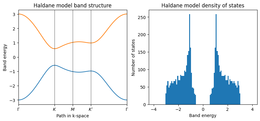
Finally, we can visualize the band structure and density of states using the obtained eigenvalues.
fig, ax = plt.subplots(1, 2, figsize=(10, 4))

ax[0].plot(k_dist, evals)
ax[0].set_xlim(k_node[0], k_node[-1])
# put tickmarks and labels at node positions
ax[0].set_xticks(k_node)
ax[0].set_xticklabels(label)
# add vertical lines at node positions
for n in range(len(k_node)):
    ax[0].axvline(x=k_node[n], linewidth=0.5, color="k")
# put title
ax[0].set_title("Haldane model band structure")
ax[0].set_xlabel("Path in k-space")
ax[0].set_ylabel("Band energy")

# now plot density of states
ax[1].hist(energies, 100, range=(-4.0, 4.0))
# ax[1].set_ylim(0.0, 80.0)
ax[1].set_title("Haldane model density of states")
ax[1].set_xlabel("Band energy")
ax[1].set_ylabel("Number of states")
Text(0, 0.5, 'Number of states')
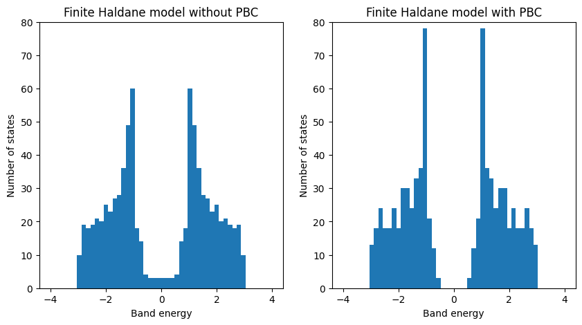
Finite Haldane model DOS#
The density of states (DOS) for the finite Haldane model can be calculated using the eigenvalues obtained from the diagonalization of the Hamiltonian. The DOS is a measure of the number of available states at each energy level and can provide insights into the electronic properties of the system.
fin_model_true = my_model.make_finite([0, 1], [20, 20], glue_edges=[True, True])
evals_true = fin_model_true.solve_ham()

fin_model_false = my_model.make_finite([0, 1], [20, 20], glue_edges=[False, False])
evals_false = fin_model_false.solve_ham()
# flatten eigenvalue arrays
evals_false = evals_false.flatten()
evals_true = evals_true.flatten()

# now plot density of states
fig, ax = plt.subplots(1, 2, figsize=(10, 5))
ax[0].hist(evals_false, 50, range=(-4.0, 4.0))
ax[0].set_ylim(0.0, 80.0)
ax[0].set_title("Finite Haldane model without PBC")
ax[0].set_xlabel("Band energy")
ax[0].set_ylabel("Number of states")

ax[1].hist(evals_true, 50, range=(-4.0, 4.0))
ax[1].set_ylim(0.0, 80.0)
ax[1].set_title("Finite Haldane model with PBC")
ax[1].set_xlabel("Band energy")
ax[1].set_ylabel("Number of states")
Text(0, 0.5, 'Number of states')