Buckled layer slab

We examine a buckled layer slab model. Orbitals live in 3D real space, but the system is periodic only in the \((x, y)\)-plane so the crystal momentum remains two-dimensional.

What you will learn

• Build a slab-style TBModel whose real space is lower dimensional than reciprocal space.

• Define a high-symmetry path in the 2D Brillouin zone for plotting.

• Compare the convenience of TBModel.plot_bands with manual diagonalization using TBModel.solve_ham.

from pythtb import TBModel, Lattice
import matplotlib.pyplot as plt

# define 3D real-space lattice vectors
lat_vecs = [[1, 0, 0], [0, 1.25, 0], [0, 0, 3]]
# define coordinates of orbitals in reduced units
orb_vecs = [[0, 0, -0.15], [0.5, 0.5, 0.15]]

# only first two lattice vectors repeat, so k-space is 2D
lat = Lattice(lat_vecs, orb_vecs, periodic_dirs=[0, 1])

my_model = TBModel(lat)

delta = 1.1
t = 0.6

# set on-site energies
my_model.set_onsite([-delta, delta])
# set hoppings (amplitude, i, j, [lattice vector to cell containing j])
my_model.set_hop(t, 1, 0, [0, 0, 0])
my_model.set_hop(t, 1, 0, [1, 0, 0])
my_model.set_hop(t, 1, 0, [0, 1, 0])
my_model.set_hop(t, 1, 0, [1, 1, 0])

print(my_model)

Show code cell output

Hide code cell output

----------------------------------------
       Tight-binding model report       
----------------------------------------
r-space dimension           = 3
k-space dimension           = 2
periodic directions         = [0, 1]
spinful                     = False
number of spin components   = 1
number of electronic states = 2
number of orbitals          = 2

Lattice vectors (Cartesian):
  # 0 ===> [ 1.000,  0.000,  0.000]
  # 1 ===> [ 0.000,  1.250,  0.000]
  # 2 ===> [ 0.000,  0.000,  3.000]
Volume of unit cell (Cartesian) = 3.750 [A^d]

Reciprocal lattice vectors (Cartesian):
  # 0 ===> [ 6.283,  0.000,  0.000]
  # 1 ===> [ 0.000,  5.027,  0.000]
Volume of reciprocal unit cell = 31.583 [A^-d]

Orbital vectors (Cartesian):
  # 0 ===> [ 0.000,  0.000, -0.450]
  # 1 ===> [ 0.500,  0.625,  0.450]

Orbital vectors (fractional):
  # 0 ===> [ 0.000,  0.000, -0.150]
  # 1 ===> [ 0.500,  0.500,  0.150]
----------------------------------------
Site energies:
  < 0 | H | 0 > = -1.100 
  < 1 | H | 1 > =  1.100 
Hoppings:
  < 1 | H | 0  + [ 0.0 ,  0.0 ,  0.0 ] > = 0.6000+0.0000j
  < 1 | H | 0  + [ 1.0 ,  0.0 ,  0.0 ] > = 0.6000+0.0000j
  < 1 | H | 0  + [ 0.0 ,  1.0 ,  0.0 ] > = 0.6000+0.0000j
  < 1 | H | 0  + [ 1.0 ,  1.0 ,  0.0 ] > = 0.6000+0.0000j
Hopping distances:
  | pos( 1 ) - pos( 0 ) + [ 0.0 ,  0.0 ,  0.0 ] | =   1.204
  | pos( 1 ) - pos( 0 ) + [ 1.0 ,  0.0 ,  0.0 ] | =   1.204
  | pos( 1 ) - pos( 0 ) + [ 0.0 ,  1.0 ,  0.0 ] | =   1.204
  | pos( 1 ) - pos( 0 ) + [ 1.0 ,  1.0 ,  0.0 ] | =   1.204

my_model.visualize_3d()

Bands along a high-symmetry path

We prescribe a sequence of nodes in the 2D Brillouin zone and let TBModel.plot_bands interpolate straight segments between them. This path will feed both plotting workflows below.

path = [[0.0, 0.0], [0.0, 0.5], [0.5, 0.5], [0.0, 0.0]]
# specify labels for these nodal points
label = (r"$\Gamma $", r"$X$", r"$M$", r"$\Gamma $")

Quick look with TBModel.plot_bands

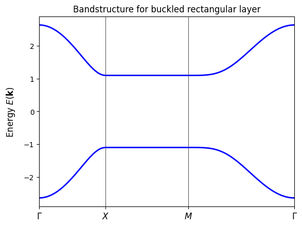
plot_bands handles path construction, diagonalization, and plotting in one call. It is great for rapid inspection of gaps, degeneracies, and orbital projections without managing k-point arrays or diagonalization manually.

fig, ax = my_model.plot_bands(k_nodes=path, k_node_labels=label, nk=100)
ax.set_title("Bandstructure for buckled rectangular layer")
plt.show()

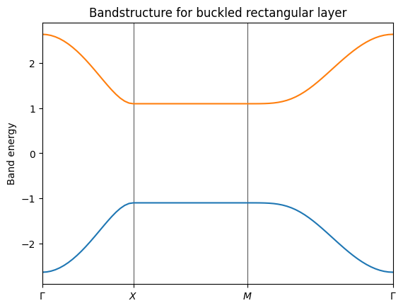
Manual diagonalization via TBModel.solve_ham

For finer control we can manually compute the interpolated k-points along path using TBModel.k_path. This will return the k-vectors along the path, the cumulative k-point distances from the first node normalized to a maximum of 1, and the cumulative distances of the high-symmetry k-points. We can then use the k-vectors to diagonalize the model.

(k_vec, k_dist, k_node) = my_model.k_path(path, 81)

evals = my_model.solve_ham(k_vec)

fig, ax = plt.subplots()
ax.set_title("Bandstructure for buckled rectangular layer")
ax.set_ylabel("Band energy")

# specify horizontal axis details
ax.set_xlim(k_node[0], k_node[-1])
# put tickmarks and labels at node positions
ax.set_xticks(k_node)
ax.set_xticklabels(label)
# add vertical lines at node positions
for n in range(len(k_node)):
    ax.axvline(x=k_node[n], linewidth=0.5, color="k")

ax.plot(k_dist, evals)
plt.show()

Next steps

Next steps

• Slice the slab with cut_piece to form a ribbon and study edge modes along the remaining periodic direction.