Edge modes in a Finite SSH chain

We sweep the Su–Schrieffer–Heeger (SSH) model from the trivial to the topological phase, tracking boundary states in a finite chain and relating them to the bulk Berry phase.

What you will learn

• Build a parameterised SSH TBModel and visualise its unit cell.

• Cut a finite chain and monitor how eigenvalues/eigenvectors evolve with hopping ratios.

• Analyze edge localization from wavefunction amplitudes.

• Compare bulk polarization via Berry phases computed with WFArray.

from pythtb import TBModel, WFArray, Mesh, Lattice
import matplotlib.pyplot as plt
import numpy as np

Model generator

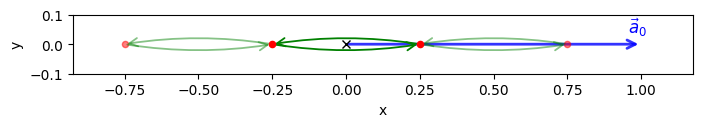
ssh(v, w) returns the periodic two-site unit cell with intracell hopping v and intercell hopping w.

Hint

pythtb.models.ssh exposes the same model function defined here.

def ssh(v, w):
    lat_vecs = [[1]]
    orb_vecs = [[-1 / 4], [1 / 4]]
    lat = Lattice(lat_vecs, orb_vecs, periodic_dirs=[0])
    my_model = TBModel(lat)

    my_model.set_hop(v, 0, 1, [0])
    my_model.set_hop(w, 1, 0, [1])

    return my_model

model = ssh(v=1, w=1 / 2)
model.visualize()

(<Figure size 800x800 with 1 Axes>, <Axes: xlabel='x', ylabel='y'>)

Finite chain sweep

For each intercell hopping \(w\) we cut a chain of n_cells unit cells, diagonalize it, and stash both eigenvalues and eigenvectors to analyse edge behaviour.

t = 1
n_cells = 30
n_delta = 101
delta_values = np.linspace(-1, 1, n_delta)

evals_d = []
evecs_d = []
for delta in delta_values:
    v = t + delta
    w = t - delta
    finite_model = ssh(v, w).cut_piece(n_cells, 0)
    evals, evecs = finite_model.solve_ham(return_eigvecs=True)
    evals_d.append(evals)
    evecs_d.append(evecs)

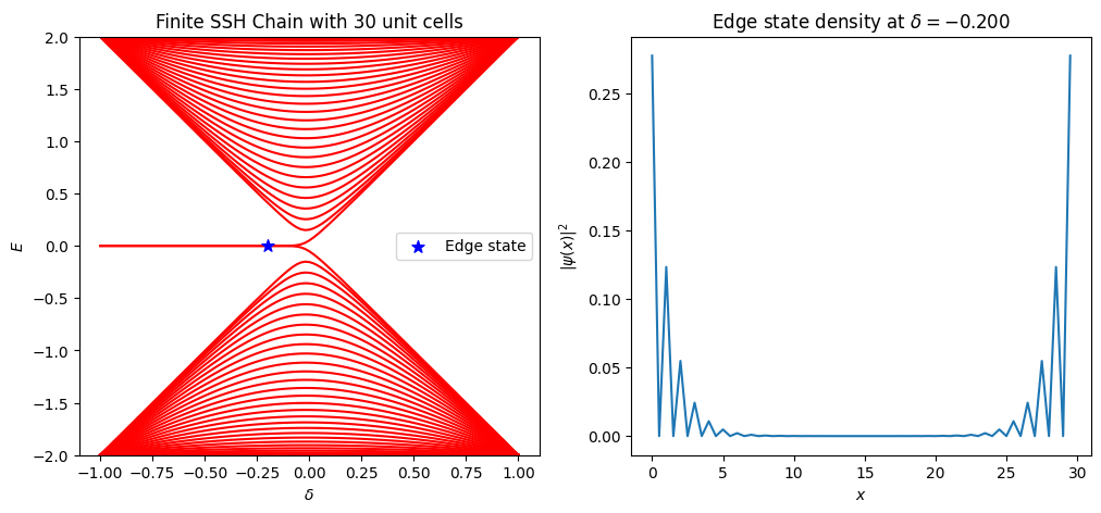
The dispersion versus \(w\) reveals a pair of mid-gap levels once \(|w| > |v|\). Evaluating the wavefunction of one of those states confirms that it is exponentially localised at the boundary.

fig, (ax1, ax2) = plt.subplots(1, 2, figsize=(12, 5))

# Plot the eigenvalues
ax1.plot(delta_values, evals_d, c="r")

ax1.set_title(f"Finite SSH Chain with {n_cells} unit cells")
ax1.set_xlabel(r"$\delta$")
ax1.set_ylabel(r"$E$")
ax1.set_ylim(-2, 2)

# Plot edge state density
band_idx = n_cells
delta_idx = 40
ax1.scatter(
    delta_values[delta_idx],
    evals_d[delta_idx][band_idx],
    color="b",
    s=70,
    marker="*",
    label="Edge state",
    zorder=2,
)
ax1.legend()
density = np.abs(evecs_d[delta_idx][band_idx, :]) ** 2
x_position = np.arange(len(density)) / 2
ax2.plot(x_position, density)
ax2.set_xlabel(r"$x$")
ax2.set_ylabel(r"$|\psi(x)|^2$")
ax2.set_title(rf"Edge state density at $\delta={delta_values[delta_idx]:.3f}$")

Text(0.5, 1.0, 'Edge state density at $\\delta=-0.200$')

Bulk polarization from Berry phases

We compare the Berry-phase-derived polarizations for the trivial (\(|w| < |v|\)) and topological (\(|w| > |v|\)) regimes using a 1D \(k\)-mesh and WFArray.berry_phase. Values are reported modulo the lattice constant.

nk = 100
mesh = Mesh(["k"])
mesh.build_grid(shape=(nk,), gamma_centered=True)

v = 1.0
model_triv = ssh(v, 0.2)
model_top = ssh(v, 1.2)
lattice = model_triv.lattice

wfa_triv = WFArray(lattice, mesh)
wfa_triv.solve_model(model_triv)
P_triv = wfa_triv.berry_phase(0, [0]) / (2 * np.pi)

wfa_top = WFArray(model_top.lattice, mesh)
wfa_top.solve_model(model_top)
P_top = wfa_top.berry_phase(0, [0]) / (2 * np.pi)

print(f"Polarization |w|<|v|: {P_triv:.3f}")
print(f"Polarization |w|>|v|: {P_top:.3f}")

Polarization |w|<|v|: -0.000
Polarization |w|>|v|: 0.500

Next steps

• Sweep both hoppings on a 2D grid to map the phase boundary where the mid-gap modes emerge.

• Add an onsite staggered potential to break chiral symmetry and track how the edge states shift.

• Couple two SSH chains with a weak inter-chain hopping and investigate how the edge spectrum hybridises.