Graphene Dirac cone Berry phase

This example computes Berry phases for a circular path (in reduced coordinates) around the Dirac point of the graphene band structure. In order to have a well defined sign of the Berry phase, a small on-site staggered potential is added to open a gap at the Dirac point.

After computing the Berry phase around the circular loop, it also computes the integral of the Berry curvature over a small square patch in the Brillouin zone containing the Dirac point, and plots individual phases for each plaquette in the array.

from pythtb import TBModel, WFArray, Mesh, Lattice
import numpy as np
import matplotlib.pyplot as plt

First we build the tight-binding model for graphene with a staggered onsite potential.

# define lattice vectors
lat_vecs = [[1, 0], [1 / 2, np.sqrt(3) / 2]]
# define coordinates of orbitals
orb_vecs = [[1 / 3, 1 / 3], [2 / 3, 2 / 3]]

lat = Lattice(lat_vecs, orb_vecs, periodic_dirs=...)

my_model = TBModel(lattice=lat)
delta = -0.1  # small staggered onsite term
t = -1.0

# set on-site energies
my_model.set_onsite([-delta, delta])
# set hoppings (amplitude, i, j, [lattice vector to cell containing j])
my_model.set_hop(t, 0, 1, [0, 0])
my_model.set_hop(t, 1, 0, [1, 0])
my_model.set_hop(t, 1, 0, [0, 1])

print(my_model)

----------------------------------------
       Tight-binding model report       
----------------------------------------
r-space dimension           = 2
k-space dimension           = 2
periodic directions         = [0, 1]
spinful                     = False
number of spin components   = 1
number of electronic states = 2
number of orbitals          = 2

Lattice vectors (Cartesian):
  # 0 ===> [ 1.000,  0.000]
  # 1 ===> [ 0.500,  0.866]
Volume of unit cell (Cartesian) = 0.866 [A^d]

Reciprocal lattice vectors (Cartesian):
  # 0 ===> [ 6.283, -3.628]
  # 1 ===> [ 0.000,  7.255]
Volume of reciprocal unit cell = 45.586 [A^-d]

Orbital vectors (Cartesian):
  # 0 ===> [ 0.500,  0.289]
  # 1 ===> [ 1.000,  0.577]

Orbital vectors (fractional):
  # 0 ===> [ 0.333,  0.333]
  # 1 ===> [ 0.667,  0.667]
----------------------------------------
Site energies:
  < 0 | H | 0 > =  0.100 
  < 1 | H | 1 > = -0.100 
Hoppings:
  < 0 | H | 1  + [ 0.0 ,  0.0 ] > = -1.0000+0.0000j
  < 1 | H | 0  + [ 1.0 ,  0.0 ] > = -1.0000+0.0000j
  < 1 | H | 0  + [ 0.0 ,  1.0 ] > = -1.0000+0.0000j
Hopping distances:
  | pos( 0 ) - pos( 1 ) + [ 0.0 ,  0.0 ] | =   0.577
  | pos( 1 ) - pos( 0 ) + [ 1.0 ,  0.0 ] | =   0.577
  | pos( 1 ) - pos( 0 ) + [ 0.0 ,  1.0 ] | =   0.577

Circular path around Dirac cone

First we will construct the circular path of k-points around the Dirac cone.

circ_step = 31  # number of steps in the circular path
circ_center = np.array([1 / 3, 2 / 3])  # the K point
circ_radius = 0.1  # the radius of the circular path

# construct k-point coordinate on the path
kpts = []
for i in range(circ_step):
    ang = 2 * np.pi * i / (circ_step - 1)
    kpt = np.array([np.cos(ang) * circ_radius, np.sin(ang) * circ_radius])
    kpt += circ_center
    kpts.append(kpt)
kpts = np.array(kpts)

Mesh class

We will now utilize the Mesh class to store the k-points along the path around the Dirac cone.

In this case, we have a one-dimensional k-path in a two-dimensional Brillouin zone, so we must specify dim_k=2 when initializing the Mesh object. We pass a single ‘k’ to the axis_types argument since we only have one k-axis in our mesh.

mesh = Mesh(["k"], dim_k=2)
mesh.build_custom(kpts)
print(mesh)

Mesh Summary
========================================
Type: path
Dimensionality: 2 k-dim(s) + 0 λ-dim(s)
Number of mesh points: 31
Full shape: (31, 2)
k-axes: [Axis(type=k, name=k_0, size=31)]
λ-axes: []
Loops: (axis 0, comp 0, winds_bz=no, closed=yes), (axis 0, comp 1, winds_bz=no, closed=yes)

WFArray class

We now construct a WFArray object to hold the wavefunction data for each k-point in the mesh. The WFArray class is designed to work seamlessly with the Mesh class, allowing us to easily associate wavefunction data with the specific k-points (or parameter points) stored in the Mesh.

w_circ = WFArray(my_model.lattice, mesh)

To populate the WFArray object with wavefunction data, we can use the solve_mesh() method, which computes the wavefunctions for each k-point in the mesh.

w_circ.solve_model(my_model)

Berry phase

We can compute the Berry phase along the circular path using the berry_phase method of the WFArray object. This method takes a list of band indices as input and returns the Berry phase for those bands.

berry_phase_0 = w_circ.berry_phase(0, [0])
berry_phase_1 = w_circ.berry_phase(0, [1])
berry_phase_both = w_circ.berry_phase(0, [0, 1])

print(
    f"Berry phase along circle with radius {circ_radius} and centered at k-point {circ_center}"
)
print(f"for band 0 equals     : {berry_phase_0: .7f}")
print(f"for band 1 equals     : {berry_phase_1: .7f}")
print(f"for both bands equals : {berry_phase_both: .7f}")

Berry phase along circle with radius 0.1 and centered at k-point [0.33333333 0.66666667]
for band 0 equals     :  2.5636831
for band 1 equals     : -2.5636831
for both bands equals :  0.0000000

Square patch around Dirac cone

Next, we construct a two-dimensional square patch covering the Dirac cone. We will construct the side length of the square patch such that the area of the patch equals the area enclosed by the loop around the Dirac point with radius circ_radius constructed above (square_length = \(\sqrt{\pi \texttt{circ\_radius}^2}\))

square_step = 50
square_center = np.array([1 / 3, 2 / 3])
square_length = np.sqrt(np.pi * circ_radius**2)

all_kpt = np.zeros((square_step, square_step, 2))
for i in range(square_step):
    for j in range(square_step):
        kpt = np.array(
            [
                square_length * (-0.5 + i / (square_step - 1)),
                square_length * (-0.5 + j / (square_step - 1)),
            ]
        )
        kpt += square_center
        all_kpt[i, j, :] = kpt

Mesh class

Added in version 2.0.0.

Again, we add the k-points into the Mesh object, but this time by calling the build_grid method. In circumstances where we have a regular grid of k-points, this method is particularly useful as it can automatically generate the necessary k-point coordinates based on the specified grid parameters. We can also specify the grid directly by passing the points parameter.

Warning

The points array must have a shape that corresponds to shape_k. For example, if shape_k is (4, 4), then points should have the shape (4, 4, 2) to represent the k-point coordinates in 2D.

mesh = Mesh(["k", "k"])
mesh.build_custom(points=all_kpt)
print(mesh)

Mesh Summary
========================================
Type: grid
Dimensionality: 2 k-dim(s) + 0 λ-dim(s)
Number of mesh points: 2500
Full shape: (50, 50, 2)
k-axes: [Axis(type=k, name=k_0, size=50), Axis(type=k, name=k_1, size=50)]
λ-axes: []
Is a torus in k-space (all k-axes wind BZ): no
Loops: None

WFArray class

Now we do the same thing as before to solve the model on these k-points, by calling solve_k_mesh on the WFArray object.

w_square = WFArray(my_model.lattice, mesh)
w_square.solve_model(my_model)

Berry flux

Next, we can compute the Berry flux on this square grid of k-points by calling WFArray.berry_flux. We pass as arguments the band indices and optionally can specify the plane on which the Berry flux should be computed.

Note

In our case, we have only one plane since the system is two-dimensional and we are interested in the Berry flux in the kx-ky plane. However, if plane is unspecified, the Berry flux will be computed for all available planes, and will be returned with an additional set of two axes corresponding to each dimension in parameter space. Since the Berry flux is an anti-symmetric tensor, the [0,1] and [1,0] components will be related by a minus sign. So here, we specify the plane so the returned object just gets the ([0,1]) component corresponding to \(\Omega(\mathbf{k})^{(0,1)}\).

b_flux_0 = w_square.berry_flux(state_idx=[0], plane=(0, 1))
b_flux_1 = w_square.berry_flux(state_idx=[1], plane=(0, 1))
b_flux_both = w_square.berry_flux(state_idx=[0, 1], plane=(0, 1))

print(
    f"Berry flux on square patch with length: {square_length} and centered at k-point: {square_center}"
)
print("for band 0 equals    : ", np.sum(b_flux_0))
print("for band 1 equals    : ", np.sum(b_flux_1))
print("for both bands equals: ", np.sum(b_flux_both))

Berry flux on square patch with length: 0.1772453850905516 and centered at k-point: [0.33333333 0.66666667]
for band 0 equals    :  2.5667991550628457
for band 1 equals    :  -2.5667991550628444
for both bands equals:  -2.6127832400890305e-15

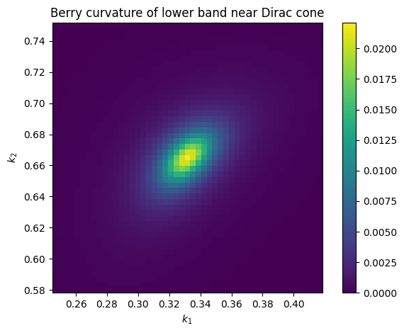
Now we will visualize the Berry flux over the square patch by plotting the individual flux for each plaquette in the grid. We expect to see a characteristic hotspot of Berry curvature centered at the Dirac point.

fig, ax = plt.subplots()
img = ax.imshow(
    b_flux_0.real,
    origin="lower",
    extent=(
        all_kpt[0, 0, 0],
        all_kpt[-2, 0, 0],
        all_kpt[0, 0, 1],
        all_kpt[0, -2, 1],
    ),
    vmax=np.amax(b_flux_0.real),
    vmin=0,
)
ax.set_title("Berry curvature of lower band near Dirac cone")
ax.set_xlabel(r"$k_1$")
ax.set_ylabel(r"$k_2$")
plt.colorbar(img)
fig.tight_layout()

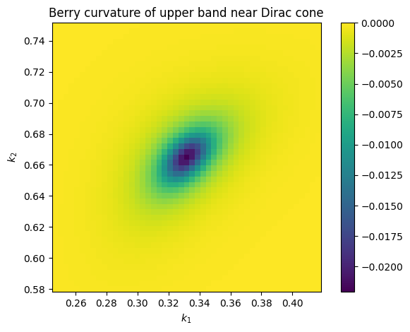
Since the model is overall time-reversal symmetric, the total Berry flux over the entire Brillouin zone must be zero. The Berry flux of the second band will be equal in magnitude but opposite in sign to that of the first band.

fig, ax = plt.subplots()
img = ax.imshow(
    b_flux_1.real,
    origin="lower",
    extent=(
        all_kpt[0, 0, 0],
        all_kpt[-2, 0, 0],
        all_kpt[0, 0, 1],
        all_kpt[0, -2, 1],
    ),
    vmax=0,
    vmin=np.amin(b_flux_1.real),
)
ax.set_title("Berry curvature of upper band near Dirac cone")
ax.set_xlabel(r"$k_1$")
ax.set_ylabel(r"$k_2$")
plt.colorbar(img)
fig.tight_layout()