Quantum geometric tensor

In this example, we examine TBModel’s berry_curvature() and quantum_metric() derived from the quantum_geometric_tensor().

TBModel can compute the quantum geometric tensor for both 2D and 3D models. Here, we illustrate its use for a 2D model. The quantum geometric tensor is defined as

\[Q_{\mu \nu;\ mn}(k) = \sum_{l \notin \text{occ}} \frac{ \langle u_{mk} | \partial_{\mu} H_k | u_{lk} \rangle \langle u_{lk} | \partial_{\nu} H_k | u_{nk} \rangle }{ (E_{mk} - E_{lk})(E_{nk} - E_{lk}) } \]

The function quantum_geometric_tensor() returns the quantum geometric tensor \(Q_{\mu \nu;\ mn}(k)\), from which the Berry curvature and quantum metric can be derived as

\[ \Omega_{\mu \nu;\ mn}(k) = i \left( Q_{\mu \nu;\ mn}(k) - Q_{\mu \nu;\ nm}^*(k) \right) \]

\[ g_{\mu \nu;\ mn}(k) = \frac{1}{2} \left( Q_{\mu \nu;\ mn}(k) + Q_{\mu \nu;\ nm}^*(k) \right) \]

In the Abelian case (i.e., trace over band indices), these reduce to the familiar expressions for the Berry curvature and quantum metric.

\[ \Omega_{\mu \nu}(k) = -2 \mathrm{Im} \, Q_{\mu \nu}(k), \]

\[ g_{\mu \nu}(k) = \mathrm{Re} \, Q_{\mu \nu}(k), \]

import numpy as np
import matplotlib.pyplot as plt

from pythtb.models import haldane

my_model = haldane(delta=0, t1=-1.0, t2=-0.15)

# Generate k-points
nkx, nky = 20, 20
k_pts = my_model.k_uniform_mesh([nkx, nky])

Berry curvature

As of v2.0, the TBModel class has the ability to compute the velocity operator as

\[ \hbar v_\alpha = \partial_{\alpha} H_{\mathbf{k}} \]

From this, we can also compute the Berry curvature arising from band mixing,

\[ \Omega^{(\alpha,\beta)}_n = \frac{1}{\hbar}\sum_{m\neq n} \frac{\langle u_{nk}| v_{k}^{\alpha} | u_{mk} \rangle \langle u_{mk} | v_{k}^{\beta}| u_{nk}\rangle}{(E_{mk} - E_{nk})^2} \]

In v1.8, the Berry curvature was only accessible through the WFArray class using the plaquette approach. Now, we can compute it directly from the TBModel.

There are a few notable features of this berry curvature implementation:

• The Berry curvature is computed using the Kubo formula above, which captures inter-band contributions to the Berry curvature. This assumes a global gap between the band of interest and all other bands. The bands of interest are specified using the occ_idxs argument.

• The Berry curvature is computed at arbitrary k-points, which we generate using the k_uniform_mesh function.

• There is a cartesian parameter to specify whether the output Berry curvature is dimensionful or in reduced units.

• There is a plane parameter to specify the 2D plane in k-space over which to compute the Berry curvature. If not specified, the returned array’s first two axes correspond to the indices of the reciprocal lattice vector directions.

• The Berry curvature has a flag for non_abelian computation, which allows one to compute the non-band-traced Berry curvature for a manifold of bands.

The full shape structure is (dim_k, dim_k, n_k, n_occ, n_occ) for the non-abelian case, and (dim_k, dim_k, n_k) for the abelian (band-traced) case.

b_curv_na = my_model.berry_curvature(
    k_pts=k_pts, occ_idxs=[0], cartesian=True, non_abelian=True
)
print(b_curv_na.shape)

(2, 2, 400, 1, 1)

By definition \(\Omega_{ij} = -\Omega_{ji}\) and \(\Omega_{ii} =0\), so we should always expect berry_curv[i,i] = 0 and berry_curv[i,j] = -berry_curv[j,i].

print(np.allclose(b_curv_na[0, 1], -b_curv_na[1, 0]))  # should be True
print(np.allclose(b_curv_na[0, 0], 0))  # should be True
print(np.allclose(b_curv_na[1, 1], 0))  # should be True

True
True
True

TBModel allows us to obtain a Chern number for a gapped manifold of states using the above Berry curvature implementation. In this case, we can compute the Chern numbers for the upper and lower bands.

.. note:: For higher-dimensional k-space systems, we should specify the 2D plane in k-space over which to compute the Chern number using the plane argument.

print(
    "Chern number band 0:",
    my_model.chern_number(plane=(0, 1), nks=(200, 200), occ_idxs=[0]),
)
print(
    "Chern number band 1:",
    my_model.chern_number(plane=(0, 1), nks=(200, 200), occ_idxs=[1]),
)

Chern number band 0: 1.0

Chern number band 1: -1.0

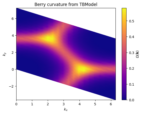
We can visualize the Berry curvature distribution for the occupied band in the two-dimensional Brillouin zone. We again call berry_curvature passing the array of k-points and occupied band indices. This time, we also specify the plane argument to indicate that we want the Berry curvature in the \((k_x, k_y)\) plane, and keep non_abelian=False to compute the band-traced Berry curvature.

b_curv = my_model.berry_curvature(
    k_pts=k_pts, plane=(0, 1), occ_idxs=[0], cartesian=True
)
print(b_curv.shape)

(400,)

To plot the Berry curvature on the reciprocal lattice, we must convert our dimensionless k-mesh to a dimensionful one. We will also reshape the berry curvature to have axes along each reciprocal lattice direction instead of being flattened

k_pts_sq = k_pts.reshape((nkx, nky, 2))
b_curv_sq = b_curv.reshape((nkx, nky))

recip_lat_vecs = my_model.recip_lat_vecs
mesh_Cart = k_pts_sq @ recip_lat_vecs

KX = mesh_Cart[:, :, 0]
KY = mesh_Cart[:, :, 1]

im = plt.pcolormesh(KX, KY, abs(b_curv_sq).real, cmap="plasma", shading="gouraud")

plt.xlabel(r"$k_x$")
plt.ylabel(r"$k_y$")
plt.colorbar(label=r"$\Omega(\mathbf{k})$")
plt.title("Berry curvature from TBModel")
plt.show()

g = my_model.quantum_metric(k_pts=k_pts, occ_idxs=[0], cartesian=True)
print(g.shape)

(2, 2, 400)

tr_g = g[0, 0] + g[1, 1]
det_g = g[0, 0] * g[1, 1] - g[0, 1] * g[1, 0]

tr_g_sq = tr_g.reshape((nkx, nky))
im = plt.pcolormesh(KX, KY, tr_g_sq.real, cmap="plasma", shading="gouraud")

plt.xlabel(r"$k_x$")
plt.ylabel(r"$k_y$")
plt.colorbar(label=r"$\text{Tr}\ g(\mathbf{k})$")
plt.title("Quantum Metric from TBModel")
plt.show()

We can assert that the weak geometric bound \(| \Omega_{xy} | \leq \text{Tr}\ g\) holds everywhere.

np.all(abs(b_curv).real <= tr_g.real)

np.False_

As well as the strong bound \(\frac{1}{4}| \Omega_{xy} |^2 \leq \ \text{det}\ g\)

np.amax((1 / 4) * abs(b_curv).real ** 2 - det_g.real)

np.float64(4.163336342344337e-17)