Graphene neighbor-shell hoppings

This graphene model calculation illustrates a case where one can use TBModel.set_nn_hops to set the n’th nearest neighbor hoppings.

from pythtb import TBModel, Lattice
import numpy as np

lat_vecs = [[1, 0], [1 / 2, np.sqrt(3) / 2]]
orb_vecs = [[1 / 3, 1 / 3], [2 / 3, 2 / 3]]

lat = Lattice(lat_vecs, orb_vecs, periodic_dirs=[0, 1])

First nearest neighbor hopping

For reference, we first create a graphene tight-binding model with only nearest neighbor hoppings.

nn_model = TBModel(lat)

shell_hops = {1: -np.exp(-1)}
nn_model.set_shell_hops(shell_hops=shell_hops, mode="set")

N’th neighbor hopping

We will now create a graphene tight-binding model and set the hopping amplitudes for the first five nearest neighbors. To do this we will use the set_shell_hops method of the TBModel class. This method takes a dictionary where the keys are the shell numbers (1 for nearest neighbor, 2 for next nearest neighbor, etc.) and the values are the hopping amplitudes.

model = TBModel(lat)

N = 5
shell_hops = {i + 1: -np.exp(-i) for i in range(N)}
model.set_shell_hops(shell_hops=shell_hops, mode="set")

print(model)

Show code cell output

Hide code cell output

----------------------------------------
       Tight-binding model report       
----------------------------------------
r-space dimension           = 2
k-space dimension           = 2
periodic directions         = [0, 1]
spinful                     = False
number of spin components   = 1
number of electronic states = 2
number of orbitals          = 2

Lattice vectors (Cartesian):
  # 0 ===> [ 1.000,  0.000]
  # 1 ===> [ 0.500,  0.866]
Volume of unit cell (Cartesian) = 0.866 [A^d]

Reciprocal lattice vectors (Cartesian):
  # 0 ===> [ 6.283, -3.628]
  # 1 ===> [ 0.000,  7.255]
Volume of reciprocal unit cell = 45.586 [A^-d]

Orbital vectors (Cartesian):
  # 0 ===> [ 0.500,  0.289]
  # 1 ===> [ 1.000,  0.577]

Orbital vectors (fractional):
  # 0 ===> [ 0.333,  0.333]
  # 1 ===> [ 0.667,  0.667]
----------------------------------------
Site energies:
  < 0 | H | 0 > =  0.000 
  < 1 | H | 1 > =  0.000 
Hoppings:
  < 0 | H | 1  + [ 0.0 , -1.0 ] > = -1.0000+0.0000j
  < 0 | H | 1  + [ 0.0 ,  0.0 ] > = -1.0000+0.0000j
  < 0 | H | 1  + [-1.0 ,  0.0 ] > = -1.0000+0.0000j
  < 0 | H | 0  + [ 1.0 ,  0.0 ] > = -0.3679+0.0000j
  < 0 | H | 0  + [-1.0 ,  1.0 ] > = -0.3679+0.0000j
  < 0 | H | 0  + [ 0.0 ,  1.0 ] > = -0.3679+0.0000j
  < 1 | H | 1  + [ 0.0 , -1.0 ] > = -0.3679+0.0000j
  < 1 | H | 1  + [-1.0 ,  0.0 ] > = -0.3679+0.0000j
  < 1 | H | 1  + [ 1.0 , -1.0 ] > = -0.3679+0.0000j
  < 0 | H | 1  + [ 1.0 , -1.0 ] > = -0.1353+0.0000j
  < 0 | H | 1  + [-1.0 ,  1.0 ] > = -0.1353+0.0000j
  < 0 | H | 1  + [-1.0 , -1.0 ] > = -0.1353+0.0000j
  < 0 | H | 1  + [ 1.0 ,  0.0 ] > = -0.0498+0.0000j
  < 0 | H | 1  + [ 1.0 , -2.0 ] > = -0.0498+0.0000j
  < 0 | H | 1  + [-2.0 ,  0.0 ] > = -0.0498+0.0000j
  < 0 | H | 1  + [-2.0 ,  1.0 ] > = -0.0498+0.0000j
  < 0 | H | 1  + [ 0.0 , -2.0 ] > = -0.0498+0.0000j
  < 0 | H | 1  + [ 0.0 ,  1.0 ] > = -0.0498+0.0000j
  < 0 | H | 0  + [-2.0 ,  1.0 ] > = -0.0183+0.0000j
  < 0 | H | 0  + [-1.0 , -1.0 ] > = -0.0183+0.0000j
  < 0 | H | 0  + [ 1.0 , -2.0 ] > = -0.0183+0.0000j
  < 1 | H | 1  + [ 1.0 , -2.0 ] > = -0.0183+0.0000j
  < 1 | H | 1  + [ 1.0 ,  1.0 ] > = -0.0183+0.0000j
  < 1 | H | 1  + [-2.0 ,  1.0 ] > = -0.0183+0.0000j
Hopping distances:
  | pos( 0 ) - pos( 1 ) + [ 0.0 , -1.0 ] | =   0.577
  | pos( 0 ) - pos( 1 ) + [ 0.0 ,  0.0 ] | =   0.577
  | pos( 0 ) - pos( 1 ) + [-1.0 ,  0.0 ] | =   0.577
  | pos( 0 ) - pos( 0 ) + [ 1.0 ,  0.0 ] | =   1.000
  | pos( 0 ) - pos( 0 ) + [-1.0 ,  1.0 ] | =   1.000
  | pos( 0 ) - pos( 0 ) + [ 0.0 ,  1.0 ] | =   1.000
  | pos( 1 ) - pos( 1 ) + [ 0.0 , -1.0 ] | =   1.000
  | pos( 1 ) - pos( 1 ) + [-1.0 ,  0.0 ] | =   1.000
  | pos( 1 ) - pos( 1 ) + [ 1.0 , -1.0 ] | =   1.000
  | pos( 0 ) - pos( 1 ) + [ 1.0 , -1.0 ] | =   1.155
  | pos( 0 ) - pos( 1 ) + [-1.0 ,  1.0 ] | =   1.155
  | pos( 0 ) - pos( 1 ) + [-1.0 , -1.0 ] | =   1.155
  | pos( 0 ) - pos( 1 ) + [ 1.0 ,  0.0 ] | =   1.528
  | pos( 0 ) - pos( 1 ) + [ 1.0 , -2.0 ] | =   1.528
  | pos( 0 ) - pos( 1 ) + [-2.0 ,  0.0 ] | =   1.528
  | pos( 0 ) - pos( 1 ) + [-2.0 ,  1.0 ] | =   1.528
  | pos( 0 ) - pos( 1 ) + [ 0.0 , -2.0 ] | =   1.528
  | pos( 0 ) - pos( 1 ) + [ 0.0 ,  1.0 ] | =   1.528
  | pos( 0 ) - pos( 0 ) + [-2.0 ,  1.0 ] | =   1.732
  | pos( 0 ) - pos( 0 ) + [-1.0 , -1.0 ] | =   1.732
  | pos( 0 ) - pos( 0 ) + [ 1.0 , -2.0 ] | =   1.732
  | pos( 1 ) - pos( 1 ) + [ 1.0 , -2.0 ] | =   1.732
  | pos( 1 ) - pos( 1 ) + [ 1.0 ,  1.0 ] | =   1.732
  | pos( 1 ) - pos( 1 ) + [-2.0 ,  1.0 ] | =   1.732

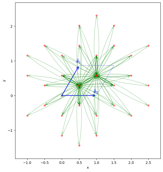
The visualize method will allow us to see the connectivity of the model after setting the hoppings.

model.visualize()

(<Figure size 800x800 with 1 Axes>, <Axes: xlabel='x', ylabel='y'>)

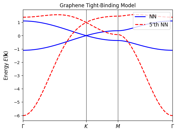
Lastly, we will plot the band structure of the model to see the effects of including up to the 5th nearest neighbor hoppings. We expect to see modifications in the band structure as we include more distant neighbor interactions.

path = [[0, 0], [2 / 3, 1 / 3], [1 / 2, 1 / 2], [0, 0]]
label = (r"$\Gamma $", r"$K$", r"$M$", r"$\Gamma $")
nk = 100

fig, ax = nn_model.plot_bands(path, label, nk, bands_label="NN", fig=None, ax=None)
model.plot_bands(
    path, label, nk, bands_label=f"{N}'th NN", fig=fig, ax=ax, ls="--", lc="r"
)
ax.set_title("Graphene Tight-Binding Model")

Text(0.5, 1.0, 'Graphene Tight-Binding Model')