Hybrid Wannier centers in the Haldane model

We revisit the Haldane Chern insulator and place the bulk Berry-phase picture in one-to-one correspondence with hybrid Wannier centers obtained from a ribbon geometry.

What you will learn

• Build a periodic model and evaluate the Berry phases,

• Cut a finite strip and solve for its edge spectrum,

• Compare hybrid Wannier centers computed in both pictures.

from pythtb import TBModel, WFArray, Lattice, Mesh
import numpy as np
import matplotlib.pyplot as plt

Build the periodic Haldane Hamiltonian

We construct a two-orbital honeycomb lattice with broken time-reversal symmetry. The TBModel is parameterized by complex second-neighbor hoppings t2 and a sublattice offset delta, yielding a Chern-insulating phase.

# define lattice vectors and orbitals and make model
lat_vecs = [[1, 0], [1 / 2, np.sqrt(3) / 2]]
orb_vecs = [[1 / 3, 1 / 3], [2 / 3, 2 / 3]]
lat = Lattice(lat_vecs, orb_vecs, periodic_dirs=...)

my_model = TBModel(lat)

# set model parameters
delta = -0.2
t = -1.0
t2 = 0.05 - 0.15j
t2c = t2.conjugate()

# set on-site energies and hoppings
my_model.set_onsite([-delta, delta])
my_model.set_hop(t, 0, 1, [0, 0])
my_model.set_hop(t, 1, 0, [1, 0])
my_model.set_hop(t, 1, 0, [0, 1])
my_model.set_hop(t2, 0, 0, [1, 0])
my_model.set_hop(t2, 1, 1, [1, -1])
my_model.set_hop(t2, 1, 1, [0, 1])
my_model.set_hop(t2c, 1, 1, [1, 0])
my_model.set_hop(t2c, 0, 0, [1, -1])
my_model.set_hop(t2c, 0, 0, [0, 1])

Discretize the Brillouin zone

The Mesh object samples both reciprocal directions with nk0 × nk1 points. This rectangular grid feeds the Berry-phase calculation and sets the resolution for the hybrid Wannier centers.

# number of discretized sites or k-points in the mesh in directions 0 and 1
nk0 = 100
nk1 = 300

mesh = Mesh(["k", "k"])
mesh.build_grid(shape=(nk0, nk1))
print(mesh)

Mesh Summary
========================================
Type: grid
Dimensionality: 2 k-dim(s) + 0 λ-dim(s)
Number of mesh points: 30000
Full shape: (100, 300, 2)
k-axes: [Axis(type=k, name=k_0, size=100), Axis(type=k, name=k_1, size=300)]
λ-axes: []
Is a torus in k-space (all k-axes wind BZ): yes
Loops: (axis 0, comp 0, winds_bz=yes, closed=no), (axis 1, comp 1, winds_bz=yes, closed=no)

Solve for the bulk Bloch states

WFArray stores eigenvalues and eigenvectors on the mesh. Solving the model populates the array with Bloch states that we will reuse for Berry phases and hybrid Wannier centers.

my_array = WFArray(lat, mesh)
my_array.solve_model(my_model)

Berry phase along a reciprocal loop

We compute the Berry phase of the valence band along the first reciprocal direction (axis_idx=0). Enabling contin=True keeps the phase evolution continuous so that the resulting hybrid Wannier center can be tracked smoothly across the Brillouin zone.

phi_0 = my_array.berry_phase(axis_idx=0, state_idx=[0], contin=True)
bulk_centers = phi_0 / (2 * np.pi)

Carve out a ribbon geometry

cut_piece turns the periodic model into a strip finite along lattice direction 0 (periodic_dir=0)and periodic along direction 1. Setting glue_edges=False removes hoppings that would connect the two edges, leaving open boundaries.

# create Haldane ribbon that is finite along direction 0
n_layers = 10
ribbon_model = my_model.cut_piece(n_layers, periodic_dir=0, glue_edges=False)

We generate a 1D momentum path parallel to the periodic direction and solve the tight-binding Hamiltonian for each point. The resulting eigenvalues and eigenvectors capture the chiral edge modes that traverse the bulk gap.

(k_vec, k_dist, k_node) = ribbon_model.k_path([0.0, 0.5, 1.0], nk1, report=False)
k_label = [r"$0$", r"$\pi$", r"$2\pi$"]

# solve ribbon model to get eigenvalues and eigenvectors
rib_eval, rib_evec = ribbon_model.solve_ham(k_vec, return_eigvecs=True)

# Fermi level, relevant for edge states of ribbon
efermi = 0.25

# shift bands so that the fermi level is at zero energy
rib_eval -= efermi

# find k-points at which number of states below the Fermi level changes
jump_k = []
for i in range(rib_eval.shape[0] - 1):
    nocc_i = np.sum(rib_eval[i, :] < 0)
    nocc_ip = np.sum(rib_eval[i + 1, :] < 0)
    if nocc_i != nocc_ip:
        jump_k.append(i)

Track orbital positions of ribbon states

For every k-point we evaluate position_expectation to obtain the average layer index of each ribbon eigenstate. States localized near opposite edges separate cleanly along the finite direction, which later guides the visual comparison. Explictly, we compute

\[ \langle x \rangle_n (k) = \langle \psi_{n,k} | \hat{x} | \psi_{n,k} \rangle \]

We specify the direction index pos_dir=0 to compute the expectation values along the finite direction of the ribbon (first lattice vector direction).

pos_exps = []

for i in range(rib_evec.shape[0]):
    # get expectation value of the position operator for states at i-th kpoint
    pos_exp = ribbon_model.position_expectation(rib_evec[i, :], pos_dir=0)
    pos_exps.append(pos_exp)

pos_exps = np.array(pos_exps)

Extract hybrid Wannier centers

position_hwf diagonalizes the position operator on the occupied ribbon states at each k-point and returns the discrete hybrid Wannier centers. These are the finite-geometry counterparts to the bulk Berry-phase result.

# get centers of hybrid wannier functions
hwfc = [
    ribbon_model.position_hwf(
        rib_evec[
            i, rib_eval[i, :] < 0.0
        ],  # get occupied states only (those below Fermi level)
        pos_dir=0,
    )
    for i in range(rib_evec.shape[0])
]

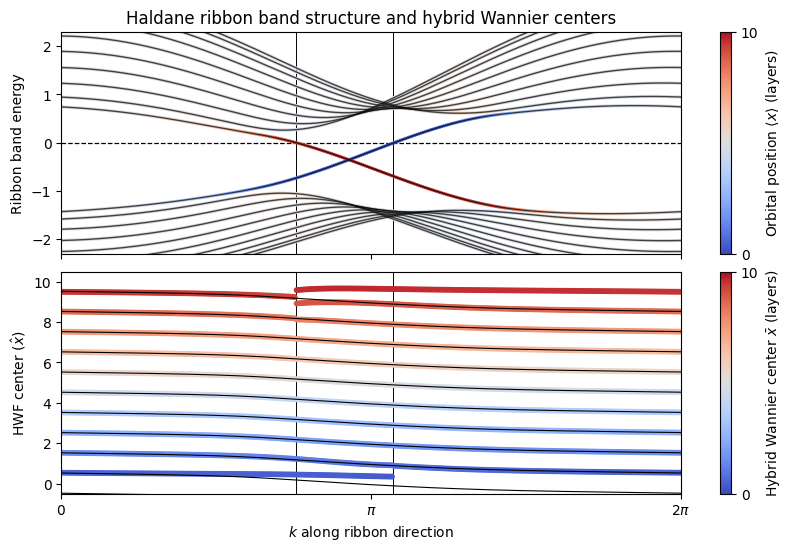
Compare bulk and ribbon viewpoints

The figure below juxtaposes the two perspectives:

• Top panel – Ribbon band structure. Thin black curves show the raw bands, while the color of the overlaid markers encodes the expectation value of the orbital position along the finite direction (⟨x⟩). Values near 0 correspond to the left edge; values near n_layers trace the right edge. The dashed horizontal line denotes the chosen Fermi level.

• Bottom panel – Hybrid Wannier information. Continuous black lines are the bulk hybrid Wannier centers (with periodic images) obtained from the Berry phase. Colored markers are the discrete centers extracted from the ribbon; their color reuses the layer-based scale. Vertical dashed guides indicate k-points where edge modes cross the Fermi level.

See also

Fig. 3 in Phys. Rev. Lett. 102, 107603 (2009).

Show code cell source

Hide code cell source

fig, (ax1, ax2) = plt.subplots(
    2,
    1,
    figsize=(10, 6),
    gridspec_kw={"height_ratios": (1.0, 1.0), "hspace": 0.08},
    sharex=True,
)

# plot bandstructure of the ribbon
ax1.plot(k_dist, rib_eval, c="k", alpha=0.7, lw=1, zorder=2)

# plot band structure with position expec. coloring
for band in range(rib_eval.shape[1]):
    sc = ax1.scatter(
        k_dist,
        rib_eval[:, band],
        c=pos_exps[:, band],
        cmap="coolwarm",
        vmin=0,
        vmax=float(n_layers),
        s=2,
        marker="o",
        zorder=1,
    )

# color scale
cbar_band = fig.colorbar(sc, ax=ax1, ticks=[0.0, float(n_layers)])
cbar_band.set_label(r"Orbital position $\langle x \rangle$ (layers)")

# plot Fermi energy
ax1.axhline(0.0, c="k", ls="--", lw=0.9, zorder=0)

# vertical lines show crossings of surface bands with Fermi energy
for ax in [ax1, ax2]:
    for i in jump_k:
        ax.axvline(
            x=(k_dist[i] + k_dist[i + 1]) / 2, linewidth=0.7, color="k", zorder=0
        )

ax1.set_title("Haldane ribbon band structure and hybrid Wannier centers")
ax1.set_ylabel("Ribbon band energy")
ax1.set_ylim(-2.3, 2.3)

# plot bulk hybrid Wannier center positions and their periodic images
for j in range(-1, n_layers + 1):
    ax2.plot(k_dist, j + bulk_centers, "k-", lw=0.8, zorder=2)

# plot finite centers of ribbon along direction 0
for i in range(rib_evec.shape[0]):
    # plot centers
    s = ax2.scatter(
        [k_dist[i]] * hwfc[i].shape[0],
        hwfc[i],
        c=hwfc[i],
        s=18,
        marker="o",
        cmap="coolwarm",
        edgecolors="none",
        vmin=0.0,
        vmax=float(n_layers),
        zorder=1,
    )

cbar_hwf = fig.colorbar(s, None, ax2, ticks=[0, float(n_layers)])
cbar_hwf.set_label(r"Hybrid Wannier center $\bar{x}$ (layers)")

ax2.set_ylabel(r"HWF center ($\hat{x}$)")
ax2.set_ylim(-0.5, n_layers + 0.5)
ax2.set_yticks(range(0, n_layers + 1, max(1, n_layers // 5)))

ax2.set_xlabel(r"$k$ along ribbon direction")
ax2.set_xlim(k_node[0], k_node[-1])
ax2.set_xticks(k_node)
ax2.set_xticklabels(k_label)
plt.show()