Bianco-Resta Local Chern marker

We compute the Bianco–Resta local Chern marker for a finite Haldane patch: first verify the bulk Chern number in momentum space, then build an open-boundary supercell and map the real-space marker, trimming the boundary to recover the bulk value.

What you will learn

• Instantiate the Haldane model and verify its bulk Chern number on a Brillouin-zone mesh.

• Generate a large open-boundary patch with make_finite and evaluate the local Chern marker.

• Aggregate site-resolved markers into unit-cell values, trim edges, and estimate the bulk topological index.

• Visualize the spatial distribution of the marker.

from pythtb import Mesh, WFArray

import matplotlib.pyplot as plt
from pythtb.models import haldane

Periodic benchmark

Construct the topological Haldane model (\(\Delta=0\), \(t=1\), \(t_2=0.15\)), check its built-in Chern number, and reproduce it via WFArray on a \(50\times 50\) Monkhorst–Pack mesh.

model = haldane(0, 1, 0.15)
print(model)

----------------------------------------
       Tight-binding model report       
----------------------------------------
r-space dimension           = 2
k-space dimension           = 2
periodic directions         = [0, 1]
spinful                     = False
number of spin components   = 1
number of electronic states = 2
number of orbitals          = 2

Lattice vectors (Cartesian):
  # 0 ===> [ 1.000,  0.000]
  # 1 ===> [ 0.500,  0.866]
Volume of unit cell (Cartesian) = 0.866 [A^d]

Reciprocal lattice vectors (Cartesian):
  # 0 ===> [ 6.283, -3.628]
  # 1 ===> [ 0.000,  7.255]
Volume of reciprocal unit cell = 45.586 [A^-d]

Orbital vectors (Cartesian):
  # 0 ===> [ 0.500,  0.289]
  # 1 ===> [ 1.000,  0.577]

Orbital vectors (fractional):
  # 0 ===> [ 0.333,  0.333]
  # 1 ===> [ 0.667,  0.667]
----------------------------------------
Site energies:
  < 0 | H | 0 > =  0.000 
  < 1 | H | 1 > =  0.000 
Hoppings:
  < 0 | H | 1  + [ 0.0 ,  0.0 ] > = 1.0000+0.0000j
  < 0 | H | 1  + [-1.0 ,  0.0 ] > = 1.0000+0.0000j
  < 0 | H | 1  + [ 0.0 , -1.0 ] > = 1.0000+0.0000j
  < 0 | H | 0  + [ 1.0 ,  0.0 ] > = 0.0000+0.1500j
  < 0 | H | 0  + [-1.0 ,  1.0 ] > = 0.0000+0.1500j
  < 0 | H | 0  + [ 0.0 , -1.0 ] > = 0.0000+0.1500j
  < 1 | H | 1  + [-1.0 ,  0.0 ] > = 0.0000+0.1500j
  < 1 | H | 1  + [ 1.0 , -1.0 ] > = 0.0000+0.1500j
  < 1 | H | 1  + [ 0.0 ,  1.0 ] > = 0.0000+0.1500j
Hopping distances:
  | pos( 0 ) - pos( 1 ) + [ 0.0 ,  0.0 ] | =   0.577
  | pos( 0 ) - pos( 1 ) + [-1.0 ,  0.0 ] | =   0.577
  | pos( 0 ) - pos( 1 ) + [ 0.0 , -1.0 ] | =   0.577
  | pos( 0 ) - pos( 0 ) + [ 1.0 ,  0.0 ] | =   1.000
  | pos( 0 ) - pos( 0 ) + [-1.0 ,  1.0 ] | =   1.000
  | pos( 0 ) - pos( 0 ) + [ 0.0 , -1.0 ] | =   1.000
  | pos( 1 ) - pos( 1 ) + [-1.0 ,  0.0 ] | =   1.000
  | pos( 1 ) - pos( 1 ) + [ 1.0 , -1.0 ] | =   1.000
  | pos( 1 ) - pos( 1 ) + [ 0.0 ,  1.0 ] | =   1.000

mesh = Mesh(["k", "k"])
mesh.build_grid(shape=(50, 50))
wfa = WFArray(model.lattice, mesh)
wfa.solve_model(model)

chern_band0 = wfa.chern_number(state_idx=[0], plane=(0, 1)).item()
print(f"Chern number (valence band): {chern_band0:+.3f}")

Chern number (valence band): -1.000

Open-boundary patch

Cut a large rectangular patch by repeating the unit cell \((L_x, L_y)\) times with model.make_finite. This returns a purely real-space TBModel (no k-axes) ready for local-marker evaluation.

# Finite OBC patch: (Lx, Ly) supercell
Lx, Ly = 42, 24
finite_model = model.make_finite(periodic_dirs=[0, 1], num_cells=[Lx, Ly])

Site-resolved marker

TBModel.local_chern_marker() yields the Bianco–Resta marker per orbital. Optionally, we can also return the bulk averaged Chern number. This requires setting trim_cells to remove the edge regions where the marker rapidly varies to compensate for the bulk value. This will trim that many unit cells from each edge of the patch. The finite model must then have at least 2*trim_cells unit cells in each direction.

Tip

Increase Lx, Ly, or adjust trim_cells if the bulk average hasn’t converged.

C_local, C_bulk_avg = finite_model.local_chern_marker(
    return_bulk_avg=True, trim_cells=4
)
print(f"Trimmed bulk marker: {C_bulk_avg:+.3f}")

Trimmed bulk marker: -1.000

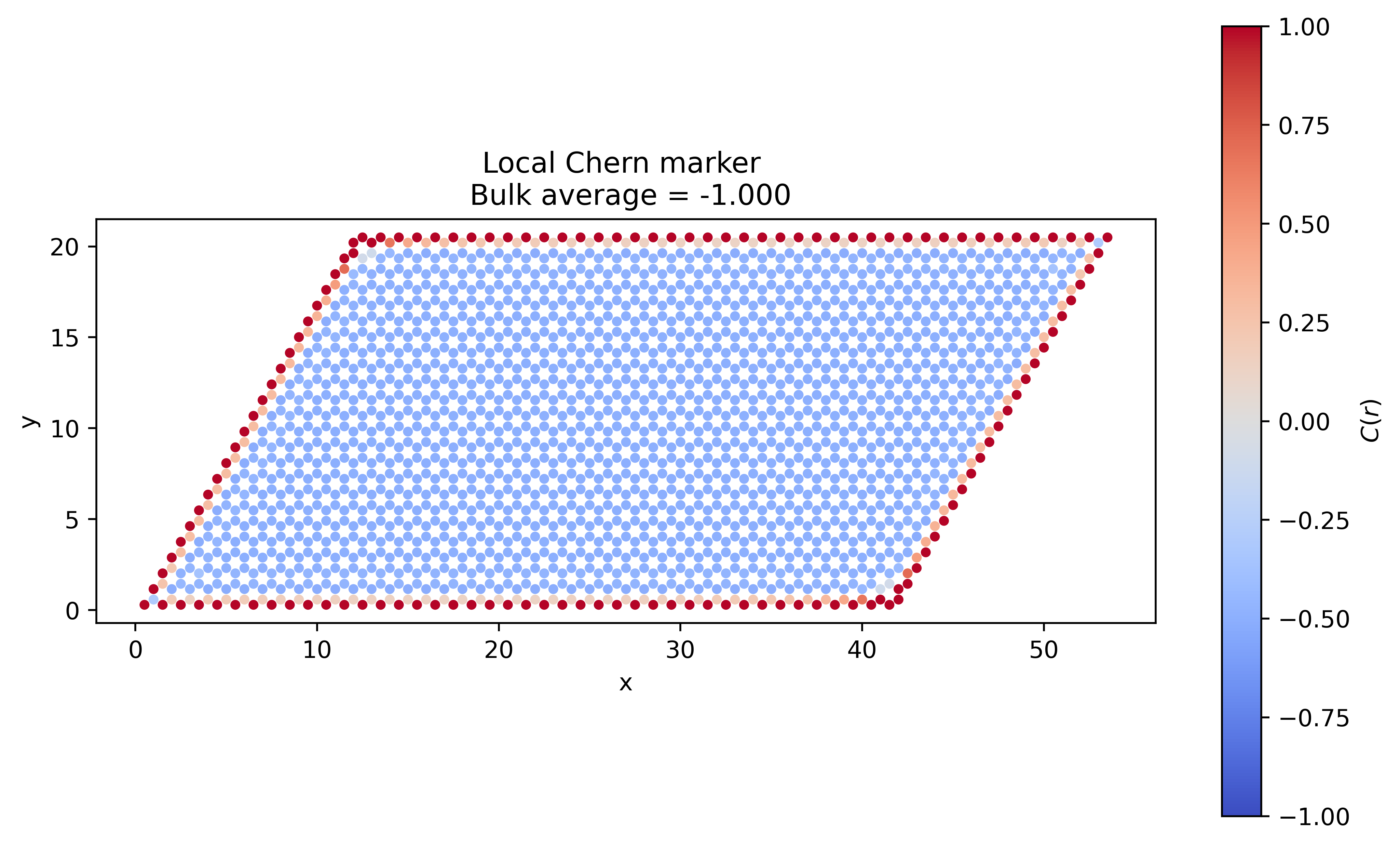
Visualize edge vs bulk

Color the orbitals by their marker value to show bulk local marker (\(\approx\) Chern number / number of sites per primitive cell) and boundary oscillations.

fig, ax = plt.subplots(figsize=(10, 6), dpi=500)
pos = finite_model.get_orb_vecs(cartesian=True)
sc = ax.scatter(
    pos[:, 0],
    pos[:, 1],
    c=C_local,
    s=10,
    cmap="coolwarm",
    vmin=-1.0,
    vmax=1.0,
)
ax.set_aspect("equal")
ax.set_xlabel("x")
ax.set_ylabel("y")
ax.set_title(f"Local Chern marker \n Bulk average = {C_bulk_avg:+.3f}")
fig.colorbar(sc, ax=ax, label=r"$C(r)$")

<matplotlib.colorbar.Colorbar at 0x79c8c91048f0>

Next steps

• Tune \((\Delta, t_2)\) to compare how the local marker behaves in the topological and trivial phases.

• Compare local_chern_marker with hybrid Wannier flow for the same finite region.