Checkerboard model#
This example shows how to define a simple two-dimensional checkerboard tight-binding model with first neighbor hopping only.
from pythtb import TBModel, Lattice
import matplotlib.pyplot as plt
Setting up the Lattice#
We start by defining the lattice vectors and the coordinates of the orbitals in fractional units. These are passed to the Lattice class to create a lattice object, along with a list of periodic directions which will be treated with periodic boundary conditions.
Note
We specify that all the lattice directions are periodic by passing periodic_dirs=.... This is a convenient shorthand for specifying all directions as periodic. Alternatively, we could have passed periodic_dirs='all', or explicitly listed periodic_dirs=[0, 1].
# define lattice vectors
lat_vecs = [[1, 0], [0, 1]]
# define coordinates of orbitals
orb_vecs = [[0, 0], [1 / 2, 1 / 2]]

lat = Lattice(lat_vecs, orb_vecs, periodic_dirs=...)
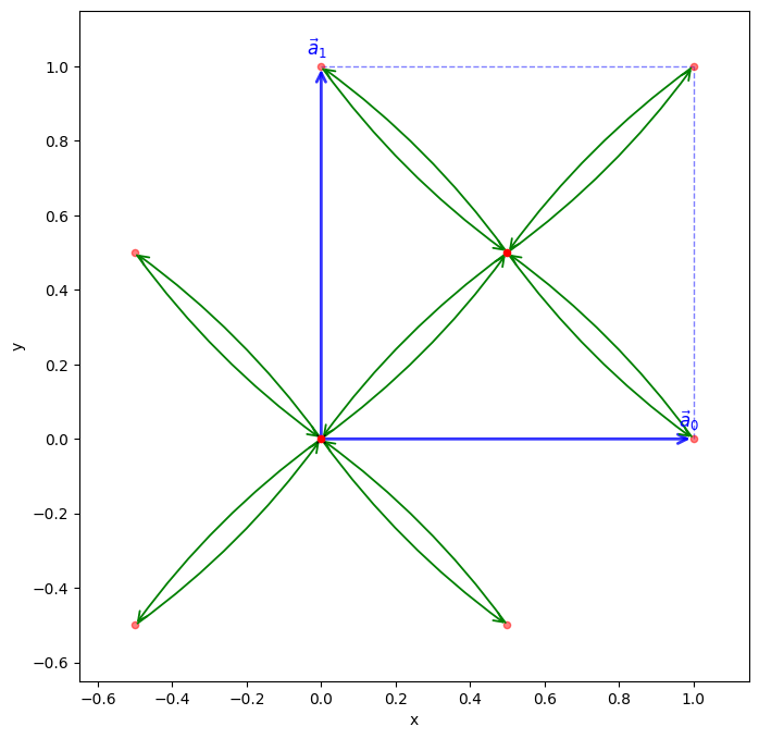
Building the TBModel#
The tight-binding model is created by passing the lattice object to the TBModel constructor. Next, the on-site energies and hopping parameters are then set using the set_onsite and set_hop methods.
my_model = TBModel(lat)

# set model parameters
delta = 1.1
t = 0.6

# set on-site energies
my_model.set_onsite([-delta, delta])
# set hoppings (one for each connected pair of orbitals)
# (amplitude, i, j, [lattice vector to cell containing j])
my_model.set_hop(t, 1, 0, [0, 0])
my_model.set_hop(t, 1, 0, [1, 0])
my_model.set_hop(t, 1, 0, [0, 1])
my_model.set_hop(t, 1, 0, [1, 1])

print(my_model)
my_model.visualize()
(<Figure size 800x800 with 1 Axes>, <Axes: xlabel='x', ylabel='y'>)
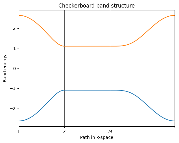
Band structure calculation#
We will now calculate the band structure of the checkerboard model by diagonalizing the tight-binding Hamiltonian on a path of k-points through the Brillouin zone. To do this, we first define the path in k-space as a list of high-symmetry points, and then use the k_path method of the TBModel class to generate the k-points along this path. Finally, we compute the band energies at each k-point using the solve_ham method and plot the resulting band structure.
path = [[0.0, 0.0], [0.0, 0.5], [0.5, 0.5], [0.0, 0.0]]
label = (r"$\Gamma $", r"$X$", r"$M$", r"$\Gamma $")
(k_vec, k_dist, k_node) = my_model.k_path(path, 301, report=True)
Now solve for eigenenergies of the Hamiltonian on the set of k-points from above. We use the k_vec array returned by k_path for this purpose. The other two arrays, k_dist and k_node, are used for plotting the band structure later on.
evals = my_model.solve_ham(k_vec)
Lastly, we plot the band structure using matplotlib.
Tip
You can use the TBModel.plot_bands method to visualize the band structure to avoid re-implementing the matplotlib code. This method takes the high-symmetry k-points defined in path as an argument and produces a plot of the energy bands.
fig, ax = plt.subplots()

ax.set_xlim(k_node[0], k_node[-1])
ax.set_xticks(k_node)
ax.set_xticklabels(label)
for n in range(len(k_node)):
    ax.axvline(x=k_node[n], linewidth=0.5, color="k")

ax.plot(k_dist, evals)

ax.set_title("Checkerboard band structure")
ax.set_xlabel("Path in k-space")
ax.set_ylabel("Band energy")
plt.show()