Boron nitride ribbon polarization#
We compare two descriptions of a boron-nitride nanoribbon: one in the original oblique unit cell, and another after reorienting the non-periodic lattice vector so it is orthogonal to the periodic direction. Both models share the same band structure, yet only the orthogonalized cell yields a Berry phase consistent with the ribbon’s physical polarization.
What you will learn
Build a 2D honeycomb model and cut out a ribbon with
TBModel.cut_piece.Re-define the non-periodic lattice vector with
TBModel.change_nonperiodic_vectorto clean up geometric invariants.Use
MeshandWFArrayto solve a 1D Brillouin-zone problem and compute Berry phases.Diagnose how cell geometry influences Wilson loops and polarization.
from pythtb import TBModel, WFArray, Mesh, Lattice
import numpy as np
import matplotlib.pyplot as plt
# define lattice vectors
lat_vecs = [[1, 0], [1 / 2, np.sqrt(3) / 2]]
# define coordinates of orbitals
orb_vecs = [[1 / 3, 1 / 3], [2 / 3, 2 / 3]]
lat = Lattice(lat_vecs, orb_vecs, periodic_dirs=...)
# make two dimensional tight-binding boron nitride model
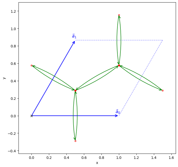
my_model = TBModel(lat)
# set periodic model
delta = 0.4
t = -1.0
my_model.set_onsite([-delta, delta])
my_model.set_hop(t, 0, 1, [0, 0])
my_model.set_hop(t, 1, 0, [1, 0])
my_model.set_hop(t, 1, 0, [0, 1])
print(my_model)
my_model.visualize()
(<Figure size 800x800 with 1 Axes>, <Axes: xlabel='x', ylabel='y'>)
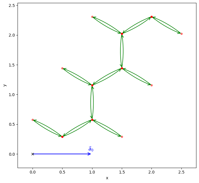
TBModel.cut_piece#
We first carve a ribbon by repeating the boron-nitride sheet three times along the second lattice vector and opening the boundary in that direction. cut_piece replicates the hoppings and onsite terms while removing the corresponding crystal-momentum axis.
model_orig = my_model.cut_piece(num_cells=3, periodic_dir=1, glue_edges=False)
print(model_orig)
model_orig.visualize()
(<Figure size 800x800 with 1 Axes>, <Axes: xlabel='x', ylabel='y'>)
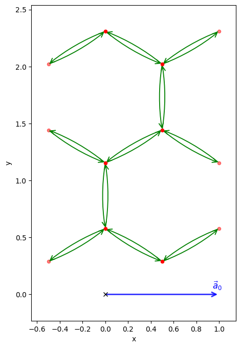
TBModel.change_nonperiodic_vector#
Next we redefine the non-periodic lattice vector so it points exactly normal to the periodic direction (default behavior). This leaves the tight-binding spectrum unchanged but simplifies the geometry that underlies Berry-phase calculations.
We first copy the original model to preserve it for comparison.
By default,
change_nonperiodic_vectororthogonalizes the non-periodic vector to the periodic one.To shift the orbitals back into the home unit cell along the periodic direction, we set
shift_orbitals=True.We can visualize these changes with
visualize()andreport().
Tip
The default behavior of change_nonperiodic_vector is to orthogonalize the non-periodic vector to the periodic one. One can also specify a custom vector with the new_latt_vec argument.
model_perp = model_orig.copy()
model_perp.change_nonperiodic_vector(fin_dir=1, to_home=True)

print(model_perp)
model_perp.visualize()
(<Figure size 800x800 with 1 Axes>, <Axes: xlabel='x', ylabel='y'>)
Bands and Berry phase#
We solve both ribbon models on the same 1D \(k\)-mesh using WFArray.solve_model, verify that their band structures coincide, and then compute the Berry phase along the periodic direction using WFArray.berry_phase. The orthogonalized cell produces the expected zero Berry phase (by mirror symmetry), while the oblique cell does not.
fig, ax = plt.subplots(1, 2, figsize=(8, 4), sharey=True)


def run_model(model, panel, title):
    k_nodes = [[-0.5], [0.5]]

    model.plot_bands(k_nodes=k_nodes, nk=100, fig=fig, ax=ax[panel], lw=1)
    ax[panel].set_xticklabels([-0.5, 0.5])

    mesh = Mesh(axis_types=["k"], dim_k=model.dim_k)
    mesh.build_grid(shape=(40,), gamma_centered=True)
    wf = WFArray(model.lattice, mesh)
    wf.solve_model(model)

    n_occ = model.nstate // 2
    berry_phase = wf.berry_phase(axis_idx=0, state_idx=range(n_occ))
    ax[panel].set_title(rf"{title}: $\phi=${berry_phase: .3f}")
    ax[panel].set_xlabel(r"$k$")

    print(f"Berry Phase {title} = {berry_phase:.7f}")


run_model(model_orig, 0, "Original")
run_model(model_perp, 1, "Shifted")

ax[1].set_ylabel(None)
fig.tight_layout()
plt.show()
Berry Phase Original = -0.4425504
Berry Phase Shifted = -0.0000000
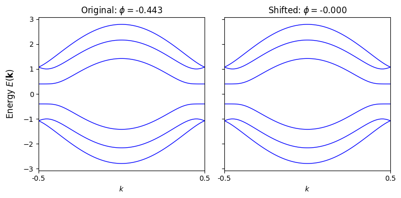
Note about mirror symmetry#
Let \(x\) denote the ribbon direction (periodic) and \(y\) the transverse direction (finite). The ribbon has an \(M_x\) mirror symmetry, so the polarization—and hence the Berry phase—must be either \(0\) or \(\pi\).
In the original oblique cell the reciprocal loop vector \(\mathbf{b}_0\) used in the Wilson loop has both \(x\) and \(y\) components. The Berry phase therefore mixes shifts of Wannier centers along \(y\) with the desired polarization along \(x\), yielding a spurious result.
After change_nonperiodic_vector, \(\mathbf{b}_0\) points purely along \(x\). The Wilson loop samples overlaps with phase factors depending only on \(x\), so the Berry phase reflects the true ribbon polarization and vanishes as dictated by symmetry. The band structure remains unchanged because it depends only on the periodic direction.
Next steps#
Next steps
Try setting
to_home=Falseinchange_nonperiodic_vectorto see how the orbital positions affect the Berry phase.Tilt the non-periodic lattice vector by a controlled angle and plot how the Berry phase deviates from the mirror-symmetric value.
Compute edge Wannier centers with
WFArray.position_expectationto visualize how the polarization migrates when the cell is oblique.