NH₃ molecular tight-binding model

This short notebook walks through a zero-dimensional tight-binding model of an ammonia (\(\text{NH}_3\)) molecule.

What you will learn

• Build a Lattice that hosts four orbitals (one on nitrogen, three on hydrogen).

• Populate a tight-binding Hamiltonian with onsite terms and uniform hoppings with TBModel.

• Visualize the bonds

• Diagonalize the Hamiltonian and inspect the molecular levels.

from pythtb import TBModel, Lattice
import numpy as np
import matplotlib.pyplot as plt

Define the molecular lattice

Even for a 0D system we provide a dummy set of lattice vectors (the identity) so PythTB can keep track of orbital positions.
The three hydrogens are arranged in a trigonal pyramid around the nitrogen.

# Cartesian axes (identity) keep the bookkeeping simple for a 0D molecule
lat_vecs = np.eye(3)

# Reduced coordinates of the four orbitals: one nitrogen at the origin, three hydrogens around it
orb_vecs = np.array(
    [
        [0, 0, 0],  # nitrogen s
        [np.sqrt(3) / 3, 0, -1],  # hydrogen s
        [-np.sqrt(3) / 6, 1 / 2, -1],  # hydrogen s
        [-np.sqrt(3) / 6, -1 / 2, -1],  # hydrogen s
    ],
    dtype=float,
)

# A finite model has no periodic directions:
# we can specify an empty list (default) or None
lat = Lattice(lat_vecs, orb_vecs, periodic_dirs=[])

Build the tight-binding Hamiltonian

We split the nitrogen onsite energy from the hydrogens with delta and keep all hoppings equal for simplicity.

Tip

Feel free to tweak delta or the hopping strength t to see how the spectrum responds.

model = TBModel(lattice=lat, spinful=False)

eps_N = -5.0  # onsite Nitrogen
eps_H = 0.0  # onsite Hydrogen
t = -2.0  # hopping N–H

# Basis defined in same order as specified orbital vectors
model.set_onsite([eps_N, eps_H, eps_H, eps_H])

# N is site 0; H sites are 1, 2, 3. Only N–H hops.
model.set_hop(t, 0, 1)
model.set_hop(t, 0, 2)
model.set_hop(t, 0, 3)

print(model)

Show code cell output

Hide code cell output

----------------------------------------
       Tight-binding model report       
----------------------------------------
r-space dimension           = 3
k-space dimension           = 0
periodic directions         = []
spinful                     = False
number of spin components   = 1
number of electronic states = 4
number of orbitals          = 4

Lattice vectors (Cartesian):
  # 0 ===> [ 1.000,  0.000,  0.000]
  # 1 ===> [ 0.000,  1.000,  0.000]
  # 2 ===> [ 0.000,  0.000,  1.000]
Volume of unit cell (Cartesian) = 1.000 [A^d]

Orbital vectors (Cartesian):
  # 0 ===> [ 0.000,  0.000,  0.000]
  # 1 ===> [ 0.577,  0.000, -1.000]
  # 2 ===> [-0.289,  0.500, -1.000]
  # 3 ===> [-0.289, -0.500, -1.000]

Orbital vectors (fractional):
  # 0 ===> [ 0.000,  0.000,  0.000]
  # 1 ===> [ 0.577,  0.000, -1.000]
  # 2 ===> [-0.289,  0.500, -1.000]
  # 3 ===> [-0.289, -0.500, -1.000]
----------------------------------------
Site energies:
  < 0 | H | 0 > = -5.000 
  < 1 | H | 1 > =  0.000 
  < 2 | H | 2 > =  0.000 
  < 3 | H | 3 > =  0.000 
Hoppings:
  < 0 | H | 1 > = -2.0000+0.0000j
  < 0 | H | 2 > = -2.0000+0.0000j
  < 0 | H | 3 > = -2.0000+0.0000j
Hopping distances:
  | pos( 0 ) - pos( 1 ) | =   1.155
  | pos( 0 ) - pos( 2 ) | =   1.155
  | pos( 0 ) - pos( 3 ) | =   1.155

The summary above confirms four orbitals, no periodic directions, and the onsite/hopping configuration we expect.
Let’s visualize the connectivity to verify the symmetry.

model.visualize_3d()

Diagonalize the Hamiltonian

TBModel.solve_ham() returns the molecular eigenvalues (and eigenvectors if requested).
We display the spectrum and annotate the bonding/antibonding character.

evals, evecs = model.solve_ham(return_eigvecs=True)

fig, ax = plt.subplots()

ax.plot(range(1, len(evals) + 1), evals, "o", color="#1f77b4")
ax.axhline(0.0, linestyle="--", color="0.7", linewidth=1)

ax.set_xticks(range(1, len(evals) + 1))
# ax.set_xticklabels([r"$E_1$", r"$E_2$", r"$E_3$", r"$E_4$"])
ax.set_xlim(0.5, len(evals) + 0.5)
ax.set_ylabel("Energy (arb. units)")
ax.set_title("NH$_3$ molecular energy levels")
plt.show()

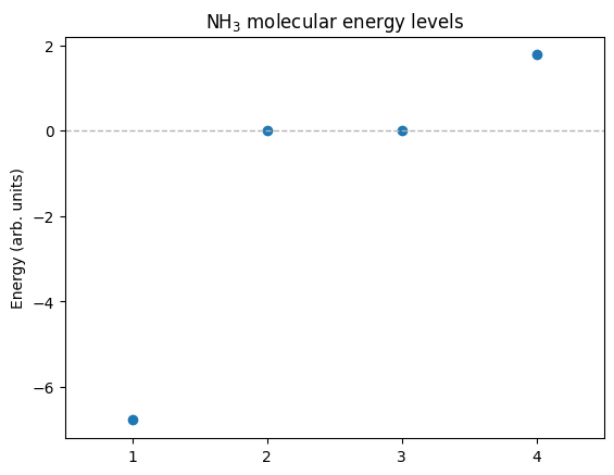
Energy levels (minimal \(\text{NH}_3\) TB model)

With one N orbital and three H orbitals (only N–H hopping \(t\)), the (\(\text{C}_{3v}\)) symmetry yields:

• \(\text{A}_1\) bonding (lowest): mixing of N with the symmetric H combination.

• \(\text{E}\) doublet (middle, twofold degenerate): non-bonding in this minimal model.

• \(\text{A}_1\) antibonding (highest).

Analytic energies:

\[ E_{\pm}=\frac{\varepsilon_N+\varepsilon_H}{2} \pm \sqrt{(\tfrac{\varepsilon_N - \varepsilon_H}{2})^2 + 3t^2}, \ \ \ E_{E}=\varepsilon_H \;\;(\text{doublet}). \]

So the spectrum is ordered: \(\text{A}_1\) (bonding) < \(\text{E}\) (doublet) < \(\text{A}_1\) (antibonding).

E_analytic_plus = (eps_N + eps_H) / 2 + np.sqrt(((eps_N - eps_H) / 2) ** 2 + 3 * t**2)
E_analytic_minus = (eps_N + eps_H) / 2 - np.sqrt(((eps_N - eps_H) / 2) ** 2 + 3 * t**2)

print(f"Analytic energies: {E_analytic_minus}, {eps_H}, {eps_H}, {E_analytic_plus}")
print(f"Computed energies: {evals[0]}, {evals[1]}, {evals[2]}, {evals[3]}")

Analytic energies: -6.772001872658765, 0.0, 0.0, 1.7720018726587652
Computed energies: -6.772001872658766, 0.0, 0.0, 1.7720018726587654

Next steps

Try

• Shift one of the hydrogen onsite energies to mimic distortions or external fields. Notice what happens to the degenerate energy levels.

• Tile \(\text{NH}_3\) units into a lattice (dim_k>0) and plot bands.

• Reduce the N–H hopping on one bond to see how the spectrum changes.

• Make spinful model spinful=True and include spin–orbit terms.