Fu-Kane–Mele 3D Topological Insulator#
A three-dimensional Fu–Kane–Mele (FKM) model on the diamond lattice realises a strong \(\mathbb{Z}_2\) topological insulator. We assemble the spinful tight-binding Hamiltonian, inspect its band structure, and trace hybrid Wannier centres that diagnose the topological phase.
What you will learn
Build the FKM Hamiltonian with first- and second-neighbour hoppings.
Plot a 3D band path and verify the insulating gap.
Sample \((k_1,k_2)\) planes at fixed \(k_3\) with
Mesh.build_custom.Compute hybrid Wannier flows with
WFArray.berry_phaseto reveal the strong TI index.
from pythtb import TBModel, WFArray, Mesh, Lattice
import matplotlib.pyplot as plt
import numpy as np
Model constructor#
The FKM Hamiltonian has the following parameters:
tsets the spin-independent nearest-neighbour hoppingdttweaks the (111) bond to break inversionsoccontrols the spin–orbit second-neighbour term.
t = 1.0  # spin-independent first-neighbor hop
dt = 0.4  # modification to t for (111) bond
soc = 0.125  # spin-dependent second-neighbor hop

lat_vecs = [[0.0, 0.5, 0.5], [0.5, 0.0, 0.5], [0.5, 0.5, 0.0]]
orb_vecs = [[0.0, 0.0, 0.0], [0.25, 0.25, 0.25]]
lattice = Lattice(lat_vecs, orb_vecs, periodic_dirs=...)
model = TBModel(lattice=lattice, spinful=True)

for lvec in ([0, 0, 0], [-1, 0, 0], [0, -1, 0], [0, 0, -1]):
    model.set_hop(t, 0, 1, lvec)
model.set_hop(dt, 0, 1, [0, 0, 0], mode="add")

lvec_list = ([1, 0, 0], [0, 1, 0], [0, 0, 1], [-1, 1, 0], [0, -1, 1], [1, 0, -1])
dir_list = ([0, 1, -1], [-1, 0, 1], [1, -1, 0], [1, 1, 0], [0, 1, 1], [1, 0, 1])
for lvec, direction in zip(lvec_list, dir_list):
    spin = np.array([0, *direction])
    model.set_hop(1j * soc * spin, 0, 0, lvec)
    model.set_hop(-1j * soc * spin, 1, 1, lvec)

print(model)
model.visualize_3d()
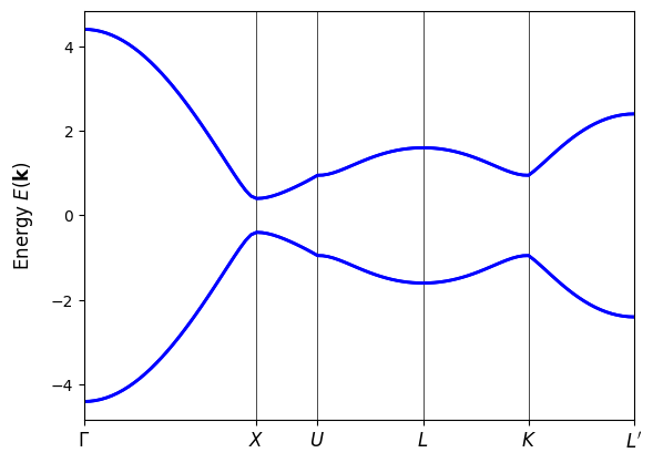
Band structure along a high-symmetry loop#
The path \(\Gamma \!\rightarrow X \!\rightarrow U \!\rightarrow L \!\rightarrow K \!\rightarrow L'\) probes the bulk Brillouin zone. TBModel.plot_bands handles interpolation and plotting so we can verify the gap.
nodes = [
    [0, 0, 0],
    [0, 1 / 2, 1 / 2],
    [1 / 4, 5 / 8, 5 / 8],
    [1 / 2, 1 / 2, 1 / 2],
    [3 / 4, 3 / 8, 3 / 8],
    [1 / 2, 0, 0],
]
label = (r"$\Gamma$", r"$X$", r"$U$", r"$L$", r"$K$", r"$L^\prime$")
model.plot_bands(k_nodes=nodes, nk=101, k_node_labels=label)
(<Figure size 640x480 with 1 Axes>, <Axes: ylabel='Energy $E(\\mathbf{{k}})$'>)
Hybrid Wannier setup#
We evaluate hybrid Wannier centers on two \((k_1,k_2)\) planes at \(k_3 = 0\) and \(k_3 = \pi\). Mesh.build_custom stacks the two slices into a single 3D mesh.
Note
Physical \((k_1,k_2,k_3)\) map to Python indices (0,1,2). Because we include the endpoints, the Brillouin-zone loops close automatically and mesh.wind_bz is unnecessary.
# number of k-points along each direction in 2D grid
nk = 101  # choose nk odd when including endpoint to include k_i = 1/2, and nk even when excluding endpoint

# To include endpoint (k_i = 1), use endpoint=True
k_vals = np.linspace(0, 1, nk, endpoint=True)

k_points = np.zeros((nk, nk, 2, 3))
for j, k2 in enumerate([0, 1 / 2]):
    for idx0, k0 in enumerate(k_vals):
        for idx1, k1 in enumerate(k_vals):
            k_points[idx0, idx1, j, :] = [k0, k1, k2]

mesh = Mesh(["k", "k", "k"])
mesh.build_custom(points=k_points)
print(mesh)
Mesh Summary
========================================
Type: grid
Dimensionality: 3 k-dim(s) + 0 λ-dim(s)
Number of mesh points: 20402
Full shape: (101, 101, 2, 3)
k-axes: [Axis(type=k, name=k_0, size=101), Axis(type=k, name=k_1, size=101), Axis(type=k, name=k_2, size=2)]
λ-axes: []
Is a torus in k-space (all k-axes wind BZ): no
Loops: (axis 0, comp 0, winds_bz=yes, closed=yes), (axis 1, comp 1, winds_bz=yes, closed=yes)
Populate WFArray on the custom mesh#
Instantiate WFArray with the lattice and mesh, then call solve_model so eigenvectors are stored at every \((k_1,k_2,k_3)\) node. These wavefunctions feed the hybrid Wannier calculation.
wfa = WFArray(model.lattice, mesh, spinful=True)
wfa.solve_model(model)
Hybrid Wannier centers#
WFArray.berry_phase(mu=1, state_idx=[0,1], contin=True, berry_evals=True) returns the Berry phases accumulated along \(k_2\) for the occupied Kramers pair. Dividing by \(2\pi\) converts them into reduced hybrid Wannier coordinates.
phi_k1 = wfa.berry_phase(axis_idx=1, state_idx=[0, 1], contin=True, berry_evals=True)
hwfc = phi_k1 / (2 * np.pi)  # hybrid Wannier charge center along k1 direction
# initialize plot
fig, ax = plt.subplots(1, 2, figsize=(12, 6), sharey=True, dpi=500)

labels = [r"$\kappa_3$=0", r"$\kappa_3$=$\pi$"]
for j in range(2):
    ax[j].set_xlim([0, 1])
    ax[j].set_xticks([0, 0.5, 1])
    ax[j].set_xticklabels([0, r"$\pi$", r"$2\pi$"])
    ax[j].set_xlabel(r"$\kappa_1$")
    ax[j].set_ylim(-0.5, 1.5)
    ax[j].text(0.08, 0.60, labels[j], size=12, bbox=dict(facecolor="w", edgecolor="k"))

    for n in range(2):
        for shift in [-1, 0, 1]:
            ax[j].plot(k_vals, hwfc[:, j, n] + shift, color="k")

ax[0].set_ylabel(r"HWF center $\bar{s}_2$", size=15)
Text(0, 0.5, 'HWF center $\\bar{s}_2$')
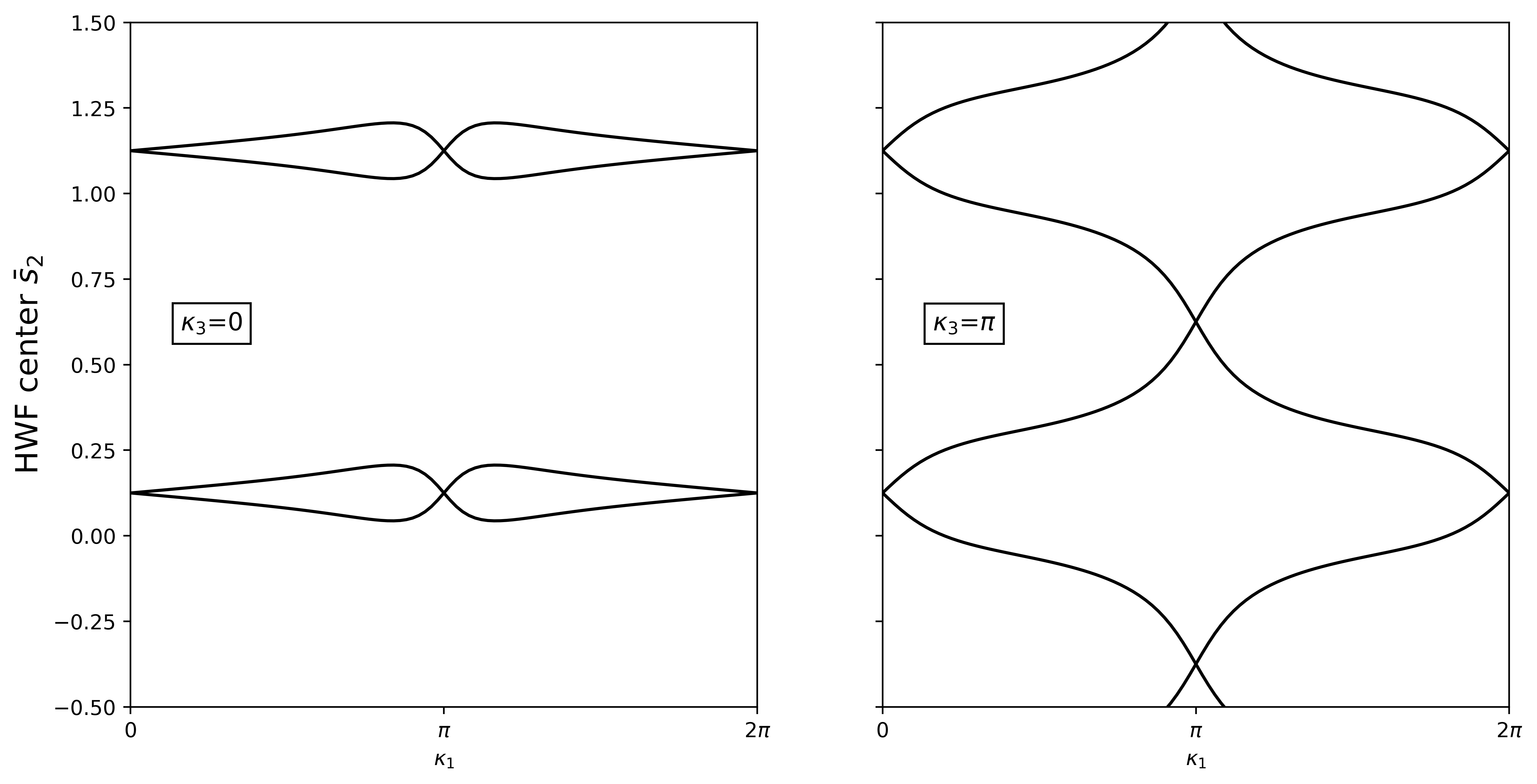
Interpreting the hybrid Wannier flow#
The hybrid Wannier flow above makes the weak \(\mathbb{Z}_2\) indices apparent:
Left panel (\(k_3 = 0\)): The two Kramers pairs meet and exchange partners exactly once as \(k_1\) winds from \(0\) to \(2\pi\). The bands reconnect without an overall shift. This tells us that the weak index \(\nu_3 = 0\).
Right panel (\(k_3 = \pi\)): Each pair winds across the unit cell, so any horizontal reference line is crossed an odd number of times in the half space \(k_1 \in [0, \pi]\). This partner-switching tells us that that the weak index \(\nu_3^\prime = 1\).
Since \(\nu_3 \neq \nu_3^\prime\), we conclude that the strong index is non-trivial \(\nu_0 = 1\) and this is a strong topological insulator.
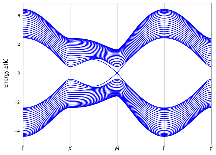
Finite slab: surface Dirac cone#
To see the bulk-boundary correspondence, we cut the Fu–Kane–Mele crystal into a slab that remains periodic in two in-plane directions but is only 20 unit cells thick along the surface normal. make_finite(periodic_dirs=[0], num_cells=[20]) keeps the \(\bar{k}_x\)–\(\bar{k}_y\) momenta and opens boundaries along the stacking axis. Plotting its surface band structure along the path \(\bar{\Gamma}\rightarrow\bar{X}\rightarrow\bar{M}\rightarrow\bar{\Gamma}\rightarrow\bar{Y}\) reveals the single gapless Dirac cone expected for a strong topological insulator.
fin_model = model.make_finite(periodic_dirs=[0], num_cells=[20])
k_nodes = [[0, 0], [0.5, 0], [0.5, 0.5], [0, 0], [0, 0.5]]
k_labels = [
    r"$\bar{\Gamma}$",
    r"$\bar{X}$",
    r"$\bar{M}$",
    r"$\bar{\Gamma}$",
    r"$\bar{Y}$",
]

fig, ax = plt.subplots(figsize=(8, 6))
fin_model.plot_bands(
    k_nodes=k_nodes, k_node_labels=k_labels, lw=1, nk=500, fig=fig, ax=ax
)
plt.show()
Next steps#
Next steps
Sweep
dtandsocto map the strong/weak TI phase boundaries.Compute Wannier center winding along other \(k\) directions to deduce the other weak indices.