Three-site Thouless pump#
We follow the three-orbital 1D Thouless pump through one adiabatic cycle, first in the periodic geometry and then as a finite chain. The onsite energies slide around the unit cell as the adiabatic parameter \(\lambda\) sweeps from 0 to 1. Along the way we track Berry phases, Wannier centres, Chern numbers, and the edge modes that reveal the pumped charge.
What you will learn
Build the periodic three-site Thouless pump with
Lattice,TBModel, andMesh.Populate a
WFArrayover a mixed \((k,\lambda)\) grid and evaluate Berry phases, Wannier centers, and Chern numbers.Cut the model to a finite chain with
cut_piece, solve its \(\lambda\)-dependent spectrum, and diagnose edge localisation viaposition_expectation.Relate the bulk Chern invariant to the pumped charge and to the edge-state crossings in the finite geometry.
import numpy as np
import matplotlib.pyplot as plt
import matplotlib

from pythtb import Lattice, Mesh, TBModel, WFArray
Lattice#
The lattice stores both the real-space lattice vectors and the three orbital positions at reduced coordinates \(0\), \(1/3\), and \(2/3\). This data is the common backbone for the TBModel and for any WFArray that samples its Bloch states.
lattice = Lattice(
    lat_vecs=[[1.0]], orb_vecs=[[0.0], [1 / 3], [2 / 3]], periodic_dirs=[0]
)
Three-site Model#
We construct the periodic three-site Hamiltonian for a given hopping t, onsite amplitude delta, and pump parameter lam. The onsite terms follow a cosine profile delayed by \(2\pi/3\) on each orbital so the deepest well moves from site 0 → 1 → 2 as \(\lambda\) advances.
We use lambda functions to define the parameterized onsite terms so that they can be evaluated later for arbitrary values of lam. The hopping terms are constant, so we set them directly with numerical values.
model = TBModel(lattice=lattice)

t = -1.3
delta = 2.0

# nearest-neighbour hoppings (last hop wraps to the next cell)
model.set_hop(t, 0, 1, [0])
model.set_hop(t, 1, 2, [0])
model.set_hop(t, 2, 0, [1])

onsite = [
    lambda lam: delta * -np.cos(2 * np.pi * (lam - 0 / 3)),
    lambda lam: delta * -np.cos(2 * np.pi * (lam - 1 / 3)),
    lambda lam: delta * -np.cos(2 * np.pi * (lam - 2 / 3)),
]

model.set_onsite(onsite)
print(model)
----------------------------------------
       Tight-binding model report
----------------------------------------
r-space dimension           = 1
k-space dimension           = 1
periodic directions         = [0]
spinful                     = False
number of spin components   = 1
number of electronic states = 3
number of orbitals          = 3

Lattice vectors (Cartesian):
  # 0 ===> [ 1.000]
Volume of unit cell (Cartesian) = 1.000 [A^d]

Reciprocal lattice vectors (Cartesian):
  # 0 ===> [ 6.283]
Volume of reciprocal unit cell = 6.283 [A^-d]

Orbital vectors (Cartesian):
  # 0 ===> [ 0.000]
  # 1 ===> [ 0.333]
  # 2 ===> [ 0.667]

Orbital vectors (fractional):
  # 0 ===> [ 0.000]
  # 1 ===> [ 0.333]
  # 2 ===> [ 0.667]
----------------------------------------
Site energies:
  < 0 | H | 0 > = lambda lam: delta * -np.cos(2 * np.pi * (lam - 0 / 3)),
  < 1 | H | 1 > = lambda lam: delta * -np.cos(2 * np.pi * (lam - 1 / 3)),
  < 2 | H | 2 > = lambda lam: delta * -np.cos(2 * np.pi * (lam - 2 / 3)),
Hoppings:
  < 0 | H | 1  + [ 0.0 ] > = -1.3000+0.0000j
  < 1 | H | 2  + [ 0.0 ] > = -1.3000+0.0000j
  < 2 | H | 0  + [ 1.0 ] > = -1.3000+0.0000j
Hopping distances:
  | pos( 0 ) - pos( 1 ) + [ 0.0 ] | =   0.333
  | pos( 1 ) - pos( 2 ) + [ 0.0 ] | =   0.333
  | pos( 2 ) - pos( 0 ) + [ 1.0 ] | =   0.333
Mesh and wavefunctions#
We sample the two-dimensional parameter space \((k,\lambda)\) with a Mesh. It is important to make sure that the adiabatic parameter \(\lambda\) is included as a parametric axis in the mesh definition. We also must ensure that the name of this parametric axis matches the keyword argument used in the onsite lambda functions, in this case "lam".
mesh = Mesh(
    dim_k=1,
    axis_types=["k", "l"],  # first axis: crystal momentum; second: adiabatic parameter
    axis_names=[
        "kx",
        "lam",
    ],  # Note: "lam" matches the variable name in the onsite functions
)
We build a uniform \((k,\lambda)\) grid and enforce periodic boundary conditions along the \(\lambda\) axis so that \(\lambda=0\) and \(\lambda=1\) are identified.
A few additional parameters are available to control the range of the parameter axis and whether to loop it.
In mesh.build_grid, we specify the start and stop values for the lambda parameter axis. By default, the endpoint is included along the lambda axes, while it is not included along the k axes. We can control this behavior with the lambda_endpoints and k_endpoints arguments.
Changed in version 2.0.0: In previous versions, mesh.loop(1,1) would have been specified in wf_array by wf_array.impose_loop(1,1). The behavior is the same.
mesh.build_grid(
    shape=(31, 21),
    gamma_centered=True,
    k_endpoints=False,
    lambda_endpoints=True,
    lambda_start=0.0,
    lambda_stop=1.0,
)

mesh.loop(axis_idx=1, component_idx=1, closed=True)  # make the lambda axis into a loop
print(mesh)
Mesh Summary
========================================
Type: grid
Dimensionality: 1 k-dim(s) + 1 λ-dim(s)
Number of mesh points: 651
Full shape: (31, 21, 2)
k-axes: [Axis(type=k, name=kx, size=31)]
λ-axes: [Axis(type=l, name=lam, size=21)]
Is a torus in k-space (all k-axes wind BZ): yes
Loops: (axis 0, comp 0, winds_bz=yes, closed=no), (axis 1, comp 1, winds_bz=no, closed=yes)
With the mesh and lattice in place, we now initialize WFArray with the lattice and mesh. We then call solve_model with the TBModel to populate the wavefunction array with the energy eigenstates over the entire \((k,\lambda)\) grid.
Note
The solve_model method of WFArray automatically imposes periodic boundary conditions on the wavefunctions.
wfa = WFArray(lattice, mesh)
wfa.solve_model(model)
Berry flux and Chern numbers#
The charge pumped per cycle equals the Chern number computed on the \((k,\lambda)\) torus. We evaluate the Berry curvature with WFArray.chern_num for individual bands and for cumulative fillings.
fillings = {
    "band 0": [0],
    "bands 0–1": [0, 1],
    "bands 0–2": [0, 1, 2],
}

cherns = {
    label: wfa.chern_number(state_idx=indices, plane=(0, 1))
    for label, indices in fillings.items()
}
band_cherns = {
    band: wfa.chern_number(state_idx=[band], plane=(0, 1)) for band in range(3)
}

print("Individual band Chern numbers:")
for band, value in band_cherns.items():
    print(f"  band {band}     = {value:+5.2f}")

print("\nChern numbers by filling:")
for label, value in cherns.items():
    print(f"  {label:<10} = {value:+5.2f}")
Individual band Chern numbers:
  band 0     = -1.00
  band 1     = +2.00
  band 2     = -1.00

Chern numbers by filling:
  band 0     = -1.00
  bands 0–1  = +1.00
  bands 0–2  = +0.00
Chern computation with Kubo formula
For comparison, we can also compute the Chern number using TBModel.chern_number, which uses a different algorithm based on the Kubo formula. The Kubo method requires a more dense mesh for the Chern number to converge to an integer than using the plaquette method, but both methods agree on the final result.
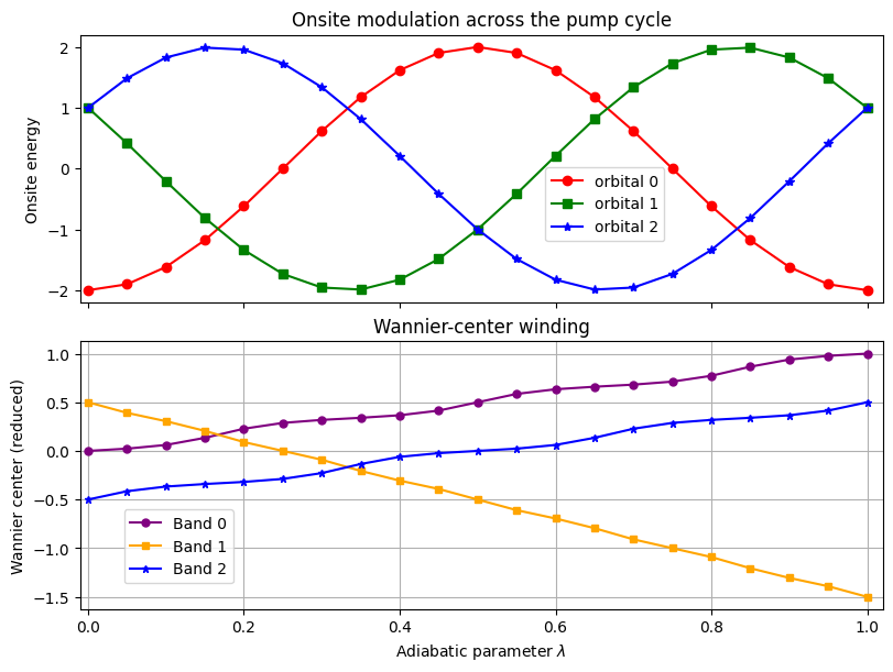
Berry phase and Wannier centers#
Another view of the pump is the Berry phase accumulated along the \(k\) axis for each \(\lambda\). Dividing that phase by \(2\pi\) gives the Wannier center in reduced coordinates; its winding number must match the band Chern number.
We compute the Abelian Berry phase for each individual band with WFArray.berry_phase and convert it to the reduced Wannier center. A single \(2\pi\) increase over the cycle signals a pumped charge of one electron per cell.
berry_phase0 = wfa.berry_phase(0, [0])
berry_phase1 = wfa.berry_phase(0, [1])
berry_phase2 = wfa.berry_phase(0, [2])

wann_center0 = berry_phase0 / (2 * np.pi)
wann_center1 = berry_phase1 / (2 * np.pi)
wann_center2 = berry_phase2 / (2 * np.pi)
fig, (ax_onsite, ax_wann) = plt.subplots(
    2, 1, figsize=(8, 6), sharex=True, constrained_layout=True
)

all_lambda = mesh.get_param_points()[:, 0]
onsite = np.vstack(
    [delta * -np.cos(2 * np.pi * (all_lambda - shift / 3.0)) for shift in range(3)]
)

ax_onsite.plot(all_lambda, onsite[0], "ro-", label="orbital 0")
ax_onsite.plot(all_lambda, onsite[1], "gs-", label="orbital 1")
ax_onsite.plot(all_lambda, onsite[2], "b*-", label="orbital 2")

ax_onsite.set_ylabel("Onsite energy")
ax_onsite.set_title("Onsite modulation across the pump cycle")
ax_onsite.legend(bbox_to_anchor=(0.57, 0.2))

ax_wann.plot(all_lambda, wann_center0, c="purple", marker="o", ms=5, label="Band 0")
ax_wann.plot(all_lambda, wann_center1, c="orange", marker="s", ms=5, label="Band 1")
ax_wann.plot(all_lambda, wann_center2, c="b", marker="*", ms=5, label="Band 2")
ax_wann.grid()
ax_wann.legend(bbox_to_anchor=(0.2, 0.4))

ax_wann.set_xlabel(r"Adiabatic parameter $\lambda$")
ax_wann.set_ylabel("Wannier center (reduced)")
ax_wann.set_xlim(-0.01, 1.02)
ax_wann.set_title("Wannier-center winding")
plt.show()
Finite chain#
To expose the edge physics behind the pump, we cut a chain of num_cells unit cells from the periodic model. cut_piece removes the \(k\) degree of freedom while keeping the hopping pattern intact.
Note
When calling cut_piece, the parametric onsite energies and hoppings are retained and translated appropriately.
num_cells = 10
num_orb = 3 * num_cells

fin_model = model.cut_piece(num_cells, periodic_dir=0)
fin_model
pythtb.TBModel(dim_r=1, dim_k=0, norb=30, spinful=False)
The finite system has no crystal momentum axis, so the mesh tracks only the adiabatic parameter. We sample \(\lambda\) densely enough to resolve the edge-state crossings.
finite_mesh = Mesh(dim_k=0, axis_types=["l"], axis_names=["lam"])
finite_mesh.build_grid(shape=(241,), lambda_start=0.0, lambda_stop=1.0)
finite_mesh.loop(0, 0, closed=True)  # lambda axis and component now indexed by 0
print(finite_mesh)
Mesh Summary
========================================
Type: grid
Dimensionality: 0 k-dim(s) + 1 λ-dim(s)
Number of mesh points: 241
Full shape: (241, 1)
k-axes: []
λ-axes: [Axis(type=l, name=lam, size=241)]
Is a torus in k-space (all k-axes wind BZ): no
Loops: (axis 0, comp 0, winds_bz=no, closed=yes)
We initialize a new WFArray on the cut lattice and solve the Hamiltonian as \(\lambda\) sweeps the cycle.
finite_wfa = WFArray(fin_model.lattice, finite_mesh)
finite_wfa.solve_model(model=fin_model)
Position expectation values#
WFArray.position_expectation(dir=0) returns the \(\langle x \rangle\) of each eigenstate in units of the lattice spacing. Bulk states cluster near the chain midpoint, while edge-localized states pin to either end.
x_expectation = finite_wfa.position_expectation(pos_dir=0)
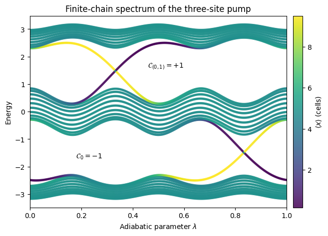
Spectrum versus \(\lambda\)#
Eigenenergies of the finite chain traced over the adiabatic cycle. Point color encodes the position expectation value \(\langle x \rangle\): bulk states (green at the chain center) stay in the gap, while edge-localized states (dark/light extremes) thread the gap and connect the valence and conduction manifolds. This matches the non-zero Chern number found for the periodic system.
lambda_points = finite_mesh.get_param_points()
vmin, vmax = x_expectation.min(), x_expectation.max()
cmap = matplotlib.colormaps.get_cmap("viridis")

fig, ax = plt.subplots(figsize=(8, 5))

for orb in range(num_orb):
    sc = ax.scatter(
        lambda_points,
        finite_wfa.energies[:, orb],
        c=x_expectation[:, orb],
        cmap=cmap,
        vmin=vmin,
        vmax=vmax,
        s=12,
        edgecolors="none",
        alpha=0.85,
    )

cbar = fig.colorbar(sc, ax=ax, pad=0.02, label=r"$\langle x \rangle$ (cells)")

ax.text(0.18, -1.7, rf"$\mathcal{{C}}_0 = {cherns['band 0']:+1.0f}$")
ax.text(0.46, 1.6, rf"$\mathcal{{C}}_{{(0,1)}} = {cherns['bands 0–1']:+1.0f}$")

ax.set_title("Finite-chain spectrum of the three-site pump")
ax.set_xlabel(r"Adiabatic parameter $\lambda$")
ax.set_ylabel("Energy")
ax.set_xlim(0.0, 1.0)

plt.show()