Berry phase and curvature in the Haldane model

In this example, we will compute the Berry phase and Berry curvature for the Haldane model on a honeycomb lattice using the pythtb package. The Haldane model is a paradigmatic example of a topological insulator in two dimensions, featuring complex next-nearest-neighbor hopping that breaks time-reversal symmetry. As such, it exhibits non-trivial topological properties characterized by a non-zero Chern number and associated Berry curvature in momentum space.

from pythtb import TBModel, Lattice, WFArray, Mesh
import numpy as np
import matplotlib.pyplot as plt

# define lattice vectors
lat_vecs = [[1, 0], [1 / 2, np.sqrt(3) / 2]]
# define coordinates of orbitals
orb_vecs = [[1 / 3, 1 / 3], [2 / 3, 2 / 3]]
lat = Lattice(lat_vecs, orb_vecs, periodic_dirs=...)

# make two dimensional tight-binding Haldane model
my_model = TBModel(lat)

# set model parameters
delta = 0
t = -1
t2 = 0.15 * np.exp(1j * np.pi / 2)
t2c = t2.conjugate()

# set on-site energies
my_model.set_onsite([-delta, delta])
# set hoppings (one for each connected pair of orbitals)
# (amplitude, i, j, [lattice vector to cell containing j])
my_model.set_hop(t, 0, 1, [0, 0])
my_model.set_hop(t, 1, 0, [1, 0])
my_model.set_hop(t, 1, 0, [0, 1])
# add second neighbour complex hoppings
my_model.set_hop(t2, 0, 0, [1, 0])
my_model.set_hop(t2, 1, 1, [1, -1])
my_model.set_hop(t2, 1, 1, [0, 1])
my_model.set_hop(t2c, 1, 1, [1, 0])
my_model.set_hop(t2c, 0, 0, [1, -1])
my_model.set_hop(t2c, 0, 0, [0, 1])

print(my_model)
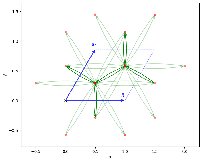
my_model.visualize()

----------------------------------------
       Tight-binding model report       
----------------------------------------
r-space dimension           = 2
k-space dimension           = 2
periodic directions         = [0, 1]
spinful                     = False
number of spin components   = 1
number of electronic states = 2
number of orbitals          = 2

Lattice vectors (Cartesian):
  # 0 ===> [ 1.000,  0.000]
  # 1 ===> [ 0.500,  0.866]
Volume of unit cell (Cartesian) = 0.866 [A^d]

Reciprocal lattice vectors (Cartesian):
  # 0 ===> [ 6.283, -3.628]
  # 1 ===> [ 0.000,  7.255]
Volume of reciprocal unit cell = 45.586 [A^-d]

Orbital vectors (Cartesian):
  # 0 ===> [ 0.500,  0.289]
  # 1 ===> [ 1.000,  0.577]

Orbital vectors (fractional):
  # 0 ===> [ 0.333,  0.333]
  # 1 ===> [ 0.667,  0.667]
----------------------------------------
Site energies:
  < 0 | H | 0 > =  0.000 
  < 1 | H | 1 > =  0.000 
Hoppings:
  < 0 | H | 1  + [ 0.0 ,  0.0 ] > = -1.0000+0.0000j
  < 1 | H | 0  + [ 1.0 ,  0.0 ] > = -1.0000+0.0000j
  < 1 | H | 0  + [ 0.0 ,  1.0 ] > = -1.0000+0.0000j
  < 0 | H | 0  + [ 1.0 ,  0.0 ] > = 0.0000+0.1500j
  < 1 | H | 1  + [ 1.0 , -1.0 ] > = 0.0000+0.1500j
  < 1 | H | 1  + [ 0.0 ,  1.0 ] > = 0.0000+0.1500j
  < 1 | H | 1  + [ 1.0 ,  0.0 ] > = 0.0000-0.1500j
  < 0 | H | 0  + [ 1.0 , -1.0 ] > = 0.0000-0.1500j
  < 0 | H | 0  + [ 0.0 ,  1.0 ] > = 0.0000-0.1500j
Hopping distances:
  | pos( 0 ) - pos( 1 ) + [ 0.0 ,  0.0 ] | =   0.577
  | pos( 1 ) - pos( 0 ) + [ 1.0 ,  0.0 ] | =   0.577
  | pos( 1 ) - pos( 0 ) + [ 0.0 ,  1.0 ] | =   0.577
  | pos( 0 ) - pos( 0 ) + [ 1.0 ,  0.0 ] | =   1.000
  | pos( 1 ) - pos( 1 ) + [ 1.0 , -1.0 ] | =   1.000
  | pos( 1 ) - pos( 1 ) + [ 0.0 ,  1.0 ] | =   1.000
  | pos( 1 ) - pos( 1 ) + [ 1.0 ,  0.0 ] | =   1.000
  | pos( 0 ) - pos( 0 ) + [ 1.0 , -1.0 ] | =   1.000
  | pos( 0 ) - pos( 0 ) + [ 0.0 ,  1.0 ] | =   1.000

(<Figure size 800x800 with 1 Axes>, <Axes: xlabel='x', ylabel='y'>)

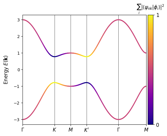
Inspect the band structure

A high-symmetry path through the hexagonal Brillouin zone highlights the gap opened by the complex second-neighbour hopping. We colour the bands by projection onto one sublattice to highlight the fact that a band-inversion occured at the \(K^\prime\) point upon the gap closing and re-opening.

k_nodes = [[0, 0], [2 / 3, 1 / 3], [0.5, 0.5], [1 / 3, 2 / 3], [0, 0], [0.5, 0.5]]
k_labels = (r"$\Gamma $", r"$K$", r"$M$", r"$K^\prime$", r"$\Gamma $", r"$M$")

my_model.plot_bands(
    k_nodes,
    k_node_labels=k_labels,
    nk=501,
    scat_size=2,
    proj_orb_idx=[1],
    cmap="plasma",
)

(<Figure size 640x480 with 2 Axes>, <Axes: ylabel='Energy $E(\\mathbf{{k}})$'>)

Brillouin-zone mesh

To compute curvature we sample the full two-dimensional Brillouin zone. Mesh(['k','k']).build_grid() builds a two-dimensional Monkhorst–Pack grid with uniform sampling.

Note

The first argument to Mesh is a list of axis types. Here we have two ‘k’ axes, indicating a 2D k-space mesh. The build_grid method then constructs the grid with the specified shape and centering. Here we specify gamma_centered=True to center the grid around the \(\Gamma\) point, meaning the k-points will range from \(-\frac{1}{2}\) to \(\frac{1}{2}\) in both directions. By default the endpoints are not included in the grid, but this can be changed with the k_endpoints argument. For the purposes of showing the winding of the hybrid Wannier centers, we will set k_endpoints=True to include the endpoints in the grid, which means the k-points will range from \(-\frac{1}{2}\) to \(\frac{1}{2}\) inclusive.

mesh = Mesh(["k", "k"])
mesh.build_grid(shape=(10, 10), gamma_centered=True, k_endpoints=[True, True])
print(mesh)

Mesh Summary
========================================
Type: grid
Dimensionality: 2 k-dim(s) + 0 λ-dim(s)
Number of mesh points: 100
Full shape: (10, 10, 2)
k-axes: [Axis(type=k, name=k_0, size=10), Axis(type=k, name=k_1, size=10)]
λ-axes: []
Is a torus in k-space (all k-axes wind BZ): yes
Loops: (axis 0, comp 0, winds_bz=yes, closed=yes), (axis 1, comp 1, winds_bz=yes, closed=yes)

Using WFArray

Generate object of type WFArray that will be used for Berry phase and curvature calculations

wfa = WFArray(my_model.lattice, mesh)
wfa.solve_model(my_model)

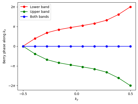
Calculate Berry phases around the BZ in the \(k_x\) direction (which can be interpreted as the 1D hybrid Wannier center in the \(x\) direction) and plot results as a function of \(k_y\).

# Berry phases along k_x for lower band
phi_0 = wfa.berry_phase(axis_idx=0, state_idx=[0], contin=True)
# Berry phases along k_x for upper band
phi_1 = wfa.berry_phase(axis_idx=0, state_idx=[1], contin=True)
# Berry phases along k_x for both bands
phi_both = wfa.berry_phase(axis_idx=0, state_idx=[0, 1], contin=True)

These results indicate that the two bands have equal and opposite Chern numbers.

# plot Berry phases
fig, ax = plt.subplots()
ky = mesh.get_axis_range(1, 1)
ax.plot(ky, phi_0, "ro-", label="Lower band")
ax.plot(ky, phi_1, "go-", label="Upper band")
ax.plot(ky, phi_both, "bo-", label="Both bands")

ax.set_xlabel(r"$k_y$")
ax.set_ylabel(r"Berry phase along $k_x$")
ax.xaxis.set_ticks([-0.5, 0, 0.5])
ax.set_ylim(-7.0, 7.0)
ax.yaxis.set_ticks([-2 * np.pi, -np.pi, 0, np.pi, 2 * np.pi])
ax.set_yticklabels((r"$-2\pi$", r"$-\pi$", r"$0$", r"$\pi$", r"$2\pi$"))
ax.legend()

<matplotlib.legend.Legend at 0x73e28ec13710>

Verify with calculation of Chern numbers

chern0 = wfa.chern_number(state_idx=[0], plane=(0, 1))
chern1 = wfa.chern_number(state_idx=[1], plane=(0, 1))

print(f"Chern number for lower band = {chern0:.11f}")
print(f"Chern number for upper band = {chern1:.11f}")

Chern number for lower band = -1.00000000000
Chern number for upper band = 1.00000000000

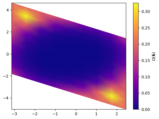
Berry flux tiles

WFArray.berry_flux(state_idx=[0], plane=(0, 1)) returns the discretized Berry flux through each plaquette for the chosen band (here the lowest). This is the gauge-invariant ingredient that sums to the band Chern number.

Note

When k_endpoints=True is used in the mesh, the Berry flux array has one fewer point in each direction than the original mesh to avoid double-counting the flux through the periodic boundary. The Berry flux is defined on the plaquettes formed by adjacent k-points, and when the endpoints are included, the last k-point is the same as the first due to periodicity.

bflux = wfa.berry_flux(state_idx=[1], plane=(0, 1))

Visualize the curvature

We map the mesh points into Cartesian momentum coordinates using the reciprocal lattice vectors, then plot the Berry flux density with pcolormesh. The peak at the \(K^\prime\) point signals the topological character of the band.

Note

Since we included the endpoints in the Mesh grid, the redundant endpoint is trimmed and the shape of the bflux array along the \(k\)-axes is (30, 30) rather than (31, 31). If an axis is sampled with \(N\) points including the endpoints, then there are only \(N-1\) plaquettes along that axis. If endpoints are excluded,

since the Berry flux is defined on the plaquettes between the k-points. The mesh.points array has shape (31, 31, 2), where the last dimension corresponds to the two momentum coordinates. This trimming is necessary to ensure that summing the Berry flux over the BZ gives the correct Chern number, which is an integer.

mesh_cart = mesh.points @ my_model.recip_lat_vecs
KX, KY = mesh_cart[..., 0], mesh_cart[..., 1]

im = plt.pcolormesh(KX[:-1, :-1], KY[:-1, :-1], bflux, cmap="plasma", shading="gouraud")
plt.colorbar(label=r"$\Omega(\mathbf{k})$")

<matplotlib.colorbar.Colorbar at 0x73e28e7e7b60>