Graphene band structure#
Graphene is a two-dimensional material with a honeycomb lattice structure. It has two atoms per unit cell, which we represent as two orbitals in our tight-binding model. We start by defining the lattice vectors and the coordinates of the orbitals in fractional units. These are passed to the Lattice class to create a lattice object, along with a list of periodic directions which will be treated with periodic boundary conditions.
Note
We specify that all the lattice directions are periodic by passing periodic_dirs=.... This is a convenient shorthand for specifying all directions as periodic. Alternatively, we could have passed periodic_dirs='all', or explicitly listed periodic_dirs=[0, 1].
from pythtb import TBModel, Lattice
import numpy as np
import matplotlib.pyplot as plt
# define lattice vectors
lat_vecs = [[1, 0], [1 / 2, np.sqrt(3) / 2]]
# define coordinates of orbitals
orb_vecs = [[1 / 3, 1 / 3], [2 / 3, 2 / 3]]
lat = Lattice(lat_vecs, orb_vecs, periodic_dirs=...)

# make two dimensional tight-binding graphene model
my_model = TBModel(lat)

# set model parameters
delta = 0.0
t = -1.0

# set on-site energies
my_model.set_onsite([-delta, delta])
# set hoppings (one for each connected pair of orbitals)
# (amplitude, i, j, [lattice vector to cell containing j])
my_model.set_hop(t, 0, 1, [0, 0])
my_model.set_hop(t, 1, 0, [1, 0])
my_model.set_hop(t, 1, 0, [0, 1])

print(my_model)
----------------------------------------
       Tight-binding model report
----------------------------------------
r-space dimension           = 2
k-space dimension           = 2
periodic directions         = [0, 1]
spinful                     = False
number of spin components   = 1
number of electronic states = 2
number of orbitals          = 2

Lattice vectors (Cartesian):
  # 0 ===> [ 1.000,  0.000]
  # 1 ===> [ 0.500,  0.866]
Volume of unit cell (Cartesian) = 0.866 [A^d]

Reciprocal lattice vectors (Cartesian):
  # 0 ===> [ 6.283, -3.628]
  # 1 ===> [ 0.000,  7.255]
Volume of reciprocal unit cell = 45.586 [A^-d]

Orbital vectors (Cartesian):
  # 0 ===> [ 0.500,  0.289]
  # 1 ===> [ 1.000,  0.577]

Orbital vectors (fractional):
  # 0 ===> [ 0.333,  0.333]
  # 1 ===> [ 0.667,  0.667]
----------------------------------------
Site energies:
  < 0 | H | 0 > = -0.000
  < 1 | H | 1 > =  0.000
Hoppings:
  < 0 | H | 1  + [ 0.0 ,  0.0 ] > = -1.0000+0.0000j
  < 1 | H | 0  + [ 1.0 ,  0.0 ] > = -1.0000+0.0000j
  < 1 | H | 0  + [ 0.0 ,  1.0 ] > = -1.0000+0.0000j
Hopping distances:
  | pos( 0 ) - pos( 1 ) + [ 0.0 ,  0.0 ] | =   0.577
  | pos( 1 ) - pos( 0 ) + [ 1.0 ,  0.0 ] | =   0.577
  | pos( 1 ) - pos( 0 ) + [ 0.0 ,  1.0 ] | =   0.577
Path in Brillouin zone from TBModel#
We generate list of k-points following a segmented path in the BZ list of nodes (high-symmetry points) using TBModel.k_path.
These high-symmetry points are specified in reduced coordinates: each entry is a list of fractional coordinates with respect to the reciprocal lattice vectors. We choose the nodes:
\(\Gamma\) =
[0, 0]\(K\) =
[2/3, 1/3]\(M\) =
[1/2, 1/2]\(\Gamma\) =
[0, 0]
Outputs:
k_path: list of interpolated k-pointsk_dist: horizontal axis position of each k-point in the listk_node_dist: horizontal axis position of each original node
k_nodes = [[0, 0], [2 / 3, 1 / 3], [1 / 2, 1 / 2], [0, 0]]
k_node_labels = (r"$\Gamma $", r"$K$", r"$M$", r"$\Gamma $")
nk = 121

k_path, k_dist, k_node_dist = my_model.k_path(k_nodes, nk)
Band structure#
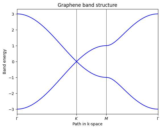
Graphene has a characteristic linear band crossing at the K point in the Brillouin zone, known as a Dirac cone. This results in unique electronic properties, such as high electron mobility and massless charge carriers. The band structure can be calculated using the tight-binding model and visualized along high-symmetry paths in the Brillouin zone.
We diagonalize the Hamiltonian at each k-point to obtain the energy eigenvalues, which represent the allowed energy levels for electrons in the material. Plotting these energy levels against the k-points gives us the band structure of graphene, revealing its electronic properties.
evals = my_model.solve_ham(k_path)
fig, ax = plt.subplots()

ax.set_xlim(k_node_dist[0], k_node_dist[-1])
ax.set_xticks(k_node_dist)
ax.set_xticklabels(k_node_labels)

for n in range(len(k_node_dist)):
    ax.axvline(x=k_node_dist[n], linewidth=0.5, color="k")

ax.set_title("Graphene band structure")
ax.set_xlabel("Path in k-space")
ax.set_ylabel("Band energy")

# plot bands
ax.plot(k_dist, evals, c="b")
plt.show()
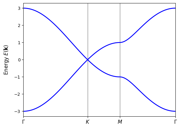
Alternatively, we can use the TBModel.band_structure method to compute the band structure directly along the specified path without having to generate the k-points separately or specify the matplotlib details. This method takes care of computing the k-points, solving the Hamiltonian, and plotting the results in one step.
my_model.plot_bands(k_nodes, k_node_labels)
plt.show()