Hybrid Wannier functions in cubic slab#
Construct and compute Berry phases of hybrid Wannier functions.
from pythtb import TBModel, Lattice, WFArray, Mesh
import matplotlib.pyplot as plt
import numpy as np
Set up model on bcc motif (CsCl structure), nearest-neighbor hopping only, but of two different strengths. Symmetry is orthorhombic with a simple \(M_y\) mirror and two diagonal mirror planes containing the \(y\) axis.
def set_model(delta, ta, tb):
    lat_vecs = [[1, 0, 0], [0, 1, 0], [0, 0, 1]]
    orb_vecs = [[0, 0, 0], [1 / 2, 1 / 2, 1 / 2]]

    model = TBModel(Lattice(lat_vecs, orb_vecs, periodic_dirs=[0, 1, 2]))

    model.set_onsite([-delta, delta])
    for lvec in ([-1, 0, 0], [0, 0, -1], [-1, -1, 0], [0, -1, -1]):
        model.set_hop(ta, 0, 1, lvec)
    for lvec in ([0, 0, 0], [0, -1, 0], [-1, -1, -1], [-1, 0, -1]):
        model.set_hop(tb, 0, 1, lvec)

    return model
delta = 1.0  # site energy shift
ta = 0.4  # six weaker hoppings
tb = 0.7  # two stronger hoppings
bulk_model = set_model(delta, ta, tb)

print(bulk_model)
bulk_model.visualize_3d()
Now make a slab model
# make slab model
num_layers = 9  # number of layers
slab_model = bulk_model.cut_piece(num_layers, 2, glue_edges=False)

# remove top orbital so top and bottom have the same termination
slab_model.remove_orb(2 * num_layers - 1)
slab_model.info(short=True)
site_colors = ["red" if i % 2 == 0 else "blue" for i in range(slab_model.norb)]
slab_model.visualize_3d(site_colors=site_colors)
# solve on grid to check insulating
nk = 10
k_1d = np.linspace(0, 1, nk, endpoint=False)
kpts = []
for kx in k_1d:
    for ky in k_1d:
        kpts.append([kx, ky])

evals = slab_model.solve_ham(kpts)

# delta > 0, so there are num_layers valence and num_layers - 1 conduction bands
en_valence = evals[:, :num_layers]
en_conduction = evals[:, num_layers + 1 :]

print(f"VB min, max = {np.min(en_valence):6.3f} , {np.max(en_valence):6.3f}")
print(f"CB min, max = {np.min(en_conduction):6.3f} , {np.max(en_conduction):6.3f}")
VB min, max = -4.447 , -1.000
CB min, max =  1.000 ,  4.447
nk = 9
mesh = Mesh(dim_k=2, axis_types=["k", "k"])
mesh.build_grid(shape=(nk, nk))
print(mesh)
Mesh Summary
========================================
Type: grid
Dimensionality: 2 k-dim(s) + 0 λ-dim(s)
Number of mesh points: 81
Full shape: (9, 9, 2)
k-axes: [Axis(type=k, name=k_0, size=9), Axis(type=k, name=k_1, size=9)]
λ-axes: []
Is a torus in k-space (all k-axes wind BZ): yes
Loops: (axis 0, comp 0, winds_bz=yes, closed=no), (axis 1, comp 1, winds_bz=yes, closed=no)
bloch_arr = WFArray(slab_model.lattice, mesh)
bloch_arr.solve_model(slab_model)
# initalize wf_array to hold HWFs, and Numpy array for HWFCs
hwf_arr = WFArray(slab_model.lattice, mesh, nstates=num_layers)
hwfc = np.zeros([nk, nk, num_layers])

# loop over k points and fill arrays with HW centers and vectors
for ix in range(nk):
    for iy in range(nk):
        (val, vec) = bloch_arr.position_hwf(
            mesh_idx=[ix, iy],
            state_idx=list(range(num_layers)),
            pos_dir=2,
            hwf_evec=True,
            basis="orbital",
        )
        hwfc[ix, iy] = val
        hwf_arr[ix, iy] = vec

# compute and print mean and standard deviation of Wannier centers by layer
print("\nLocations of hybrid Wannier centers along z:\n")
print("  Layer      " + num_layers * "  %2d    " % tuple(range(num_layers)))
print("  Mean   " + num_layers * "%8.4f" % tuple(np.mean(hwfc, axis=(0, 1))))
print("  Std Dev" + num_layers * "%8.4f" % tuple(np.std(hwfc, axis=(0, 1))))
Locations of hybrid Wannier centers along z:

  Layer         0       1       2       3       4       5       6       7       8
  Mean     0.0582  1.0097  2.0024  3.0006  4.0000  4.9994  5.9976  6.9903  7.9418
  Std Dev  0.0410  0.0114  0.0035  0.0010  0.0000  0.0010  0.0035  0.0114  0.0410
# compute and print layer contributions to polarization along x, then y
px = np.zeros((num_layers, nk))
py = np.zeros((num_layers, nk))
for n in range(num_layers):
    px[n, :] = hwf_arr.berry_phase(axis_idx=0, state_idx=[n]) / (2 * np.pi)
    py[n, :] = hwf_arr.berry_phase(axis_idx=1, state_idx=[n]) / (2 * np.pi)

print("\nBerry phases along x (rows correspond to k_y points):\n")
print("  Layer      " + num_layers * "  %2d    " % tuple(range(num_layers)))
for k in range(nk):
    print("         " + num_layers * "%8.4f" % tuple(px[:, k]))
# when averaging, don't count last k-point
px_mean = np.mean(px[:, :-1], axis=1)
py_mean = np.mean(py[:, :-1], axis=1)
print("\n  Avg P_x" + num_layers * "%8.4f" % tuple(px_mean))
Berry phases along x (rows correspond to k_y points):
Layer 0 1 2 3 4 5 6 7 8
0.0607 0.0090 0.0022 0.0006 0.0000 -0.0006 -0.0022 -0.0090 -0.0607
0.0568 0.0079 0.0018 0.0005 0.0000 -0.0005 -0.0018 -0.0079 -0.0568
0.0448 0.0048 0.0009 0.0002 -0.0000 -0.0002 -0.0009 -0.0048 -0.0448
0.0255 0.0014 0.0001 0.0000 0.0000 -0.0000 -0.0001 -0.0014 -0.0255
0.0044 0.0000 0.0000 0.0000 0.0000 -0.0000 -0.0000 -0.0000 -0.0044
0.0044 0.0000 0.0000 0.0000 -0.0000 -0.0000 -0.0000 -0.0000 -0.0044
0.0255 0.0014 0.0001 0.0000 -0.0000 -0.0000 -0.0001 -0.0014 -0.0255
0.0448 0.0048 0.0009 0.0002 0.0000 -0.0002 -0.0009 -0.0048 -0.0448
0.0568 0.0079 0.0018 0.0005 0.0000 -0.0005 -0.0018 -0.0079 -0.0568
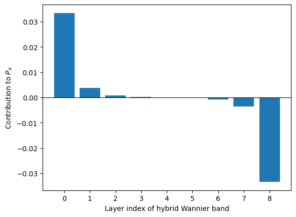
Avg P_x 0.0334 0.0037 0.0008 0.0002 0.0000 -0.0002 -0.0008 -0.0037 -0.0334
# compute and print layer contributions to polarization along x, then y
px = np.zeros((num_layers, nk))
py = np.zeros((num_layers, nk))
for n in range(num_layers):
    px[n, :] = hwf_arr.berry_phase(axis_idx=0, state_idx=[n]) / (2 * np.pi)
    py[n, :] = hwf_arr.berry_phase(axis_idx=1, state_idx=[n]) / (2 * np.pi)

print("\nBerry phases along x (rows correspond to k_y points):\n")
print("  Layer      " + num_layers * "  %2d    " % tuple(range(num_layers)))
for k in range(nk):
    print("         " + num_layers * "%8.4f" % tuple(px[:, k]))
# when averaging, don't count last k-point
px_mean = np.mean(px[:, :-1], axis=1)
py_mean = np.mean(py[:, :-1], axis=1)
print("\n  Avg P_x" + num_layers * "%8.4f" % tuple(px_mean))
Berry phases along x (rows correspond to k_y points):

  Layer         0       1       2       3       4       5       6       7       8
           0.0607  0.0090  0.0022  0.0006  0.0000 -0.0006 -0.0022 -0.0090 -0.0607
           0.0568  0.0079  0.0018  0.0005  0.0000 -0.0005 -0.0018 -0.0079 -0.0568
           0.0448  0.0048  0.0009  0.0002 -0.0000 -0.0002 -0.0009 -0.0048 -0.0448
           0.0255  0.0014  0.0001  0.0000  0.0000 -0.0000 -0.0001 -0.0014 -0.0255
           0.0044  0.0000  0.0000  0.0000  0.0000 -0.0000 -0.0000 -0.0000 -0.0044
           0.0044  0.0000  0.0000  0.0000 -0.0000 -0.0000 -0.0000 -0.0000 -0.0044
           0.0255  0.0014  0.0001  0.0000 -0.0000 -0.0000 -0.0001 -0.0014 -0.0255
           0.0448  0.0048  0.0009  0.0002  0.0000 -0.0002 -0.0009 -0.0048 -0.0448
           0.0568  0.0079  0.0018  0.0005  0.0000 -0.0005 -0.0018 -0.0079 -0.0568

  Avg P_x  0.0334  0.0037  0.0008  0.0002  0.0000 -0.0002 -0.0008 -0.0037 -0.0334
Similar calculations along \(y\) give zero due to \(M_y\) mirror symmetry.
nlh = num_layers // 2
sum_top = np.sum(py_mean[:nlh])
sum_bot = np.sum(py_mean[-nlh:])
print("\n  Surface sums: Top, Bottom = %8.4f , %8.4f\n" % (sum_top, sum_bot))
Surface sums: Top, Bottom = -0.0000 , -0.0000
These quantities are essentially the “surface polarizations” of the model as defined within the hybrid Wannier gauge.
See also
S. Ren, I. Souza, and D. Vanderbilt, “Quadrupole moments, edge polarizations, and corner charges in the Wannier representation,” Phys. Rev. B 103, 035147 (2021).
fig = plt.figure()
plt.bar(range(num_layers), px_mean)
plt.axhline(0.0, linewidth=0.8, color="k")
plt.xticks(range(num_layers))
plt.xlabel("Layer index of hybrid Wannier band")
plt.ylabel(r"Contribution to $P_x$")
Text(0, 0.5, 'Contribution to $P_x$')