Graphene neighbor-shell hoppings#
This graphene model calculation illustrates a case where one can use TBModel.set_shell_hops to set the n’th nearest neighbor hoppings.
from pythtb import TBModel, Lattice
import numpy as np
lat_vecs = [[1, 0], [1 / 2, np.sqrt(3) / 2]]
orb_vecs = [[1 / 3, 1 / 3], [2 / 3, 2 / 3]]

lat = Lattice(lat_vecs, orb_vecs, periodic_dirs=[0, 1])
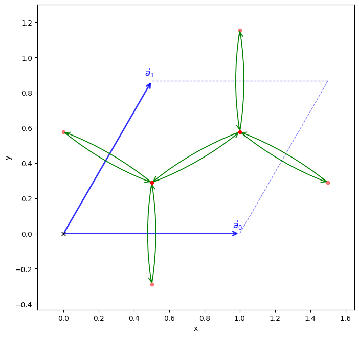
First nearest neighbor hopping#
For reference, we first create a graphene tight-binding model with only nearest neighbor hoppings.
nn_model = TBModel(lat)

shell_hops = {1: -np.exp(-1)}
nn_model.set_shell_hops(shell_hops=shell_hops, mode="set")
nn_model.visualize()
(<Figure size 800x800 with 1 Axes>, <Axes: xlabel='x', ylabel='y'>)
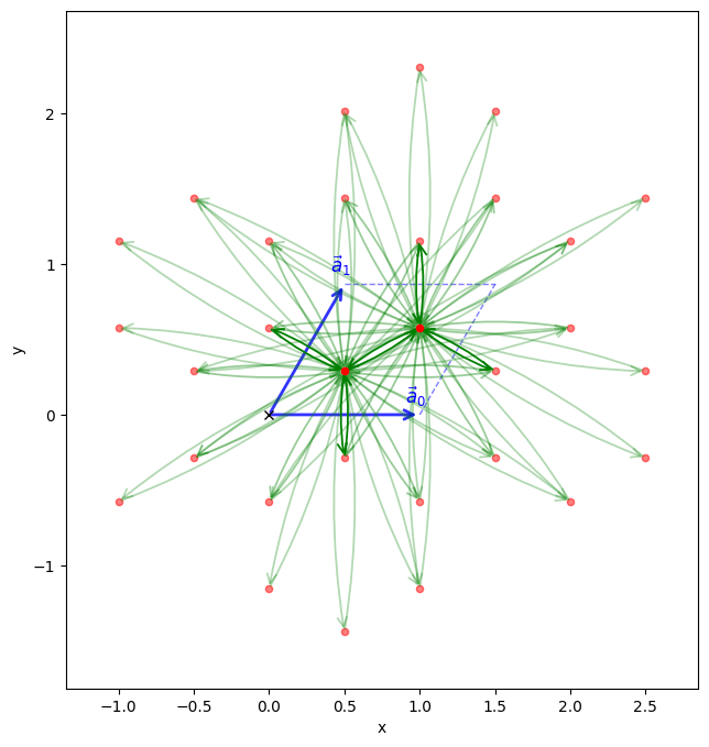
N’th neighbor hopping#
We will now create a graphene tight-binding model and set the hopping amplitudes for the first five nearest neighbors. To do this we will use the set_shell_hops method of the TBModel class. This method takes a dictionary of the form {shell: amp} where the keys are the shell numbers (1 for nearest neighbor, 2 for next nearest neighbor, etc.) and the values are the hopping amplitudes.
Setting different hoppings within the same shell
This function will set all hoppings in the specified shells to the same given values. If we want to set different hoppings within the same shell to different values, we can use the set_hop method with the information returned by nn_bonds instead.
nn_bonds returns a tuple, the first being a list of dictionaries, one for each shell, containing information about the hoppings in that shell. The second element is
a list of lists, one list for each shell. Each element of a list for a given shell is a tuple of (site_i, site_j, R_vector) identifying a hopping in that shell. The conjugate hoppings are not included, as those are handled automatically in set_hop.
We would manually loop over the shells and the hoppings within each shell to set different values as desired.
shell_bonds = self.nn_bonds(max_shell)
amp = [[...], ...]  # define hopping amplitude as desired
mode = "set"  # or "add", etc.

for shell_idx, shell in enumerate(shell_bonds[1]):
    for bond_idx, bond in enumerate(shell):
        i, j, R = bond
        self.set_hop(amp[shell_idx][bond_idx], i, j, R, mode=mode)
model = TBModel(lat)

shells = list(range(1, 6))
shell_hops = {i: -np.exp(-i) for i in shells}  # exponentially decreasing hoppings
model.set_shell_hops(shell_hops=shell_hops, mode="set")

print(model)
The visualize method will allow us to see the connectivity of the model after setting the hoppings.
model.visualize()
(<Figure size 800x800 with 1 Axes>, <Axes: xlabel='x', ylabel='y'>)
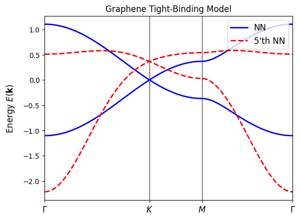
Band stucture with shells up to 5th nearest neighbor#
We now compute the band structure of graphene while progressively including hopping terms out to the 5th nearest neighbor shell. Each additional shell introduces corrections beyond the ideal nearest-neighbor model. In particular:
2nd-neighbor hoppings generate same-sublattice terms that break particle–hole symmetry,
3rd and 4th shells distort the Dirac cone and modify the trigonal warping,
higher shells potentially recover more realistic quantitative dispersions.
By comparing band structures with 1, 3, and 5 shells, we can directly visualize how distant-neighbor interactions reshape the dispersion and lift the artificial symmetries of the minimal tight-binding model.
path = [[0, 0], [2 / 3, 1 / 3], [1 / 2, 1 / 2], [0, 0]]
label = (r"$\Gamma $", r"$K$", r"$M$", r"$\Gamma $")
nk = 100

fig, ax = nn_model.plot_bands(path, label, nk, bands_label="NN", fig=None, ax=None)
model.plot_bands(
    path, label, nk, bands_label=f"{max(shells)}'th NN", fig=fig, ax=ax, ls="--", lc="r"
)
ax.set_title("Graphene Tight-Binding Model")
Text(0.5, 1.0, 'Graphene Tight-Binding Model')
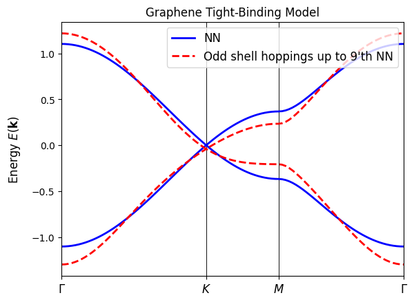
Band structure using only odd neighbor shells#
For comparison, we repeat the calculation while including only odd-indexed neighbor shells (1st, 3rd, 5th). These hoppings connect opposite sublattices and therefore preserve the particle-hole symmetry of the idealized graphene Dirac spectrum.
Because even shells (especially 2nd neighbors) introduce same-sublattice hoppings that break particle–hole symmetry, the odd-shell-only model retains a band structure that remains closer to the idealized symmetric Dirac spectrum. By examining the differences between this restricted model and the full shell expansion, we can isolate the specific role of even-shell hoppings in distorting and shifting the Dirac point.
model = TBModel(lat)

shells = [1, 3, 5, 7, 9]
shell_hops = {i: -np.exp(-i) for i in shells}  # exponentially decreasing hoppings
model.set_shell_hops(shell_hops=shell_hops, mode="set")

fig, ax = nn_model.plot_bands(path, label, nk, bands_label="NN", fig=None, ax=None)
model.plot_bands(
    path,
    label,
    nk,
    bands_label=f"Odd shell hoppings up to {max(shells)}'th NN",
    fig=fig,
    ax=ax,
    ls="--",
    lc="r",
)
ax.set_title("Graphene Tight-Binding Model")
Text(0.5, 1.0, 'Graphene Tight-Binding Model')